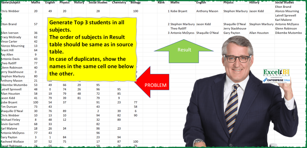
Generate Top 3 students in all subjects. The order of subjects in Result table should be same as in source table. In case of duplicates, show the names in the same cell one below the other.
📌 Challenge Details and Links
ExcelBI Power Query Challenge Number: 81
Challenge Difficulty: ⭐️⭐️⭐️⭐️
📥Download Sample File
📥Link to the solutions on LinkedIn
Solving the challenge of Top 3 Students Per Subject with Power Query
Power Query solution 1 for Top 3 Students Per Subject, proposed by Bo Rydobon 🇹🇭:
let
 Source = Excel.CurrentWorkbook(){[Name="Table1"]}[Content],
 Group = Table.FromColumns(List.Accumulate( List.Skip(Table.ColumnNames(Source)),{{1,2,3}}, (s,l)=> s& {List.FirstN(Table.Sort(Table.Group(Source, {l},
 {"C", each Text.Combine([#"NameSubject"],"#(lf)")}),{l,1})[C],3)}) , {"Rank"}&List.Skip(Table.ColumnNames(Source)))
in
 Group
Power Query solution 2 for Top 3 Students Per Subject, proposed by Zoran Milokanović:
let
 Source = Excel.CurrentWorkbook(){[Name="Input"]}[Content],
 ToColumns = {{1..3}} & List.Transform(List.Skip(Table.ToColumns(Source)), each List.Accumulate(List.Accumulate({0..2}, {}, (s, c) => s & {List.Max(List.RemoveItems(_, s))}), {}, (s, c) => s & {Text.Combine(List.Transform(List.PositionOf(_, c, 2), each Source[#"NameSubject"]{_}), "#(cr)#(lf)")})),
 Solution = Table.FromColumns(ToColumns, {"Rank"} & List.Skip(Table.ColumnNames(Source)) )
in
 Solution
Power Query solution 3 for Top 3 Students Per Subject, proposed by Kris Jaganah:
let
 Source = Excel.CurrentWorkbook(){[Name="Table1"]}[Content],
 #"Replaced Value" = Table.ReplaceValue(Source,null,0,Replacer.ReplaceValue,{"Maths", "English", "Physics", "History", "Social Studies", "Chemistry", "Biology"}),
 #"Unpivoted Other Columns" = Table.UnpivotOtherColumns(#"Replaced Value", {"NameSubject"}, "Attribute", "Value"),
 #"Added Index" = Table.AddIndexColumn(#"Unpivoted Other Columns", "Index", 1, 1, Int64.Type),
 #"Added Custom" = Table.AddColumn(#"Added Index", "Subject Rank", each if Number.Mod([Index],7)= 0 then 7 else Number.Mod([Index],7)),
 #"Grouped Rows" = Table.Group(#"Added Custom", {"Attribute"}, {{"Group", each _, type table [#"NameSubject"=text, Attribute=text, Value=number, Index=number, Subject Rank=number]}}),
 #"Added Custom1" = Table.AddColumn(#"Grouped Rows", "Custom", each Table.AddRankColumn([Group],"Rank",{"Value",Order.Descending},[RankKind=RankKind.Dense])),
 #"Removed Other Columns" = Table.SelectColumns(#"Added Custom1",{"Custom"}),
Power Query solution 4 for Top 3 Students Per Subject, proposed by Alejandro Simón 🇵🇦 🇪🇸:
let
 Source = Excel.CurrentWorkbook(){[Name="Table1"]}[Content],
 Unpivot = Table.UnpivotOtherColumns(Source, {"NameSubject"}, "Attribute", "Value"),
 Group = Table.Combine(Table.Group(Unpivot, {"Attribute"}, {{"All", each
 let
 a = Table.FirstN(Table.Sort(Table.Group(_, {"Value", "Attribute"}, {{"All", each Text.Combine([#"NameSubject"], "#(lf)")}}), {"Value", Order.Descending}), 3),
 b = Table.AddIndexColumn(a, "Rank", 1,1)
 in Table.RemoveColumns(b, "Value")}})[All]),
 Sol = Table.SelectColumns(Table.Pivot(Group, List.Distinct(Group[Attribute]), "Attribute", "All"),{"Rank"}&List.Skip(Table.ColumnNames(Source)))
in
 Sol
Power Query solution 5 for Top 3 Students Per Subject, proposed by Luan Rodrigues:
let
 Fonte = Tabela1,
 list = List.Skip(Table.ColumnNames(Fonte),1),
 col = Table.UnpivotOtherColumns(Fonte, {"NameSubject"}, "Atributo", "Valor"),
 gp = Table.Group(col, {"Atributo"}, {{"Contagem", each
 [
 a = List.MaxN(List.Distinct(_[Valor]),3),
 b = Table.AddIndexColumn(Table.Sort(Table.Group(Table.SelectRows(_, each List.Contains(a,[Valor])),{"Valor"},{{"Count", each Text.Combine(_[#"NameSubject"],", ")}}),{"Valor",Order.Descending}) ,"Rank",1,1)
 [[Rank],[Count]]
 ][b]}}),
 class = Table.Sort(gp,each List.PositionOf(list,[Atributo] ) ),
 exp = Table.ExpandTableColumn(class, "Contagem", {"Rank", "Count"}),
 res = Table.Pivot(exp, List.Distinct(exp[Atributo]), "Atributo", "Count")
in
 res
Power Query solution 6 for Top 3 Students Per Subject, proposed by Eric Laforce:
let
  Source = Excel.CurrentWorkbook(){[Name = "tData81"]}[Content],
  Columns = Table.ToColumns(Source),
  Names = Columns{0},
  Subjects = List.Skip(Table.ColumnNames(Source)),
  Transform = List.Transform(
    List.Skip(Columns),
    each
      let
        _Notes = List.Sort(List.Distinct(_), Order.Descending),
        _Ranks = List.Transform(_, each 1 + List.PositionOf(_Notes, _)),
        _RN = List.Select(List.Zip({_Ranks, Names}), each _{0} <= 3),
        _Grp = Table.Group(
          Table.FromRows(_RN, {"R", "N"}),
          "R",
          {"GN", each Text.Combine(_[N], "#(lf)")}
        )
      in
        Table.Sort(_Grp, "R")[GN]
  ),
  ToTable = Table.FromColumns({{1, 2, 3}} & Transform, {"Rank"} & Subjects)
in
  ToTable
Power Query solution 7 for Top 3 Students Per Subject, proposed by Victor Wang:
let
 Source = Excel.CurrentWorkbook(){[Name="Table1"]}[Content],
 Subjects = List.Skip(Table.ColumnNames(Source)),
 Accumulate = List.Accumulate(Subjects, {{1..3}}, (s,c)=> s & {List.Transform({1..3}, (a)=> Lines.ToText(Table.SelectRows( Table.AddRankColumn(Source, "Rank", {c,1} , [RankKind = RankKind.Dense]), (b)=> b[Rank] = a)[#"NameSubject"]))}),
 fromColumns = Table.FromColumns(Accumulate, {"Rank"} & Subjects)
in
 fromColumns
Power Query solution 9 for Top 3 Students Per Subject, proposed by Obi E, MPH:
let
 Source = Excel.CurrentWorkbook(){[Name="Table1"]}[Content],
 #"Unpivoted Columns" = Table.UnpivotOtherColumns(Source, {"NameSubject"}, "Attribute", "Value"),
 #"Grouped Rows" = Table.Group(#"Unpivoted Columns", {"Attribute"}, {{"Count", each Table.FirstN(Table.Sort(_,{{"Value", Order.Descending}}),3), type table [#"NameSubject"=text, Attribute=text, Value=number]}}),
 #"Added Custom" = Table.AddColumn(#"Grouped Rows", "Custom", each Table.AddIndexColumn([Count],"Index",1,1)),
 #"Removed Columns1" = Table.RemoveColumns(#"Added Custom",{"Count"}),
 #"Expanded Custom" = Table.ExpandTableColumn(#"Removed Columns1", "Custom", {"NameSubject", "Attribute", "Value", "Index"}, {"NameSubject", "Attribute.1", "Value", "Index"}),
 #"Removed Columns2" = Table.RemoveColumns(#"Expanded Custom",{"Attribute.1", "Value"}),
 #"Pivoted Column1" = Table.Pivot(#"Removed Columns2", List.Distinct(#"Removed Columns2"[Attribute]), "Attribute", "NameSubject")
in
 #"Pivoted Column1"
Solving the challenge of Top 3 Students Per Subject with Excel
Excel solution 1 for Top 3 Students Per Subject, proposed by Bo Rydobon 🇹🇭:
=LET(z,B2:H31,HSTACK({"Rank";1;2;3},VSTACK(B1:H1,MAKEARRAY(3,COLUMNS(z),LAMBDA(r,c,LET(s,INDEX(z,,c),TEXTJOIN("
",,FILTER(A2:A31,s=LARGE(UNIQUE(s),r)))))))))
Excel solution 2 for Top 3 Students Per Subject, proposed by محمد حلمي:
=VSTACK(HSTACK("Rank",B1:H1),HSTACK(ROW(1:3),MAKEARRAY(3,7,LAMBDA(r,c,LET(v,INDEX(B2:H31,,c),INDEX(BYCOL(
IF(v=LARGE(UNIQUE(v),{1,2,3}),A2:A31,""),
LAMBDA(a,TEXTJOIN(CHAR(10),,a))),r))))))
Excel solution 3 for Top 3 Students Per Subject, proposed by Oscar Mendez Roca Farell:
=LET(_e, B1:H1, VSTACK(HSTACK("Rank",_e), REDUCE({1; 2; 3},_e, LAMBDA(i, x, LET(b, INDEX(B2:H31, , XMATCH(x,_e)), HSTACK(i, TEXTSPLIT(TEXTJOIN(";", , BYCOL(REPT(A2:A31, b=LARGE(UNIQUE(b),{1,2,3})), LAMBDA(c, TEXTJOIN(CHAR(10), ,c)))), ,";")))))))Excel solution 4 for Top 3 Students Per Subject, proposed by Duy Tùng:
=VSTACK(HSTACK("Rank",B1:H1),REDUCE({1;2;3},B2:H2,LAMBDA(x,y,LET(a,TAKE(y:H31,,1),f,LAMBDA(v,TEXTJOIN(CHAR(10),,FILTER(A2:A31,a=LARGE(UNIQUE(a),v)))),HSTACK(x,VSTACK(f(1),f(2),f(3)))))))Excel solution 5 for Top 3 Students Per Subject, proposed by Sunny Baggu:
=VSTACK(
 HSTACK("Rank", B1:H1),
 HSTACK(
 SEQUENCE(3),
 MAKEARRAY(
 3,
 COLUMNS(B1:H1),
 LAMBDA(r, c,
 TEXTJOIN(
 CHAR(10),
 ,
 FILTER(
 A2:A31,
 INDEX(B2:H31, , c) = LARGE(UNIQUE(INDEX(B2:H31, , c)), r)
 )
 )
 )
 )
 )
)
Excel solution 6 for Top 3 Students Per Subject, proposed by Sunny Baggu:
=HSTACK(
 SEQUENCE(3),
 DROP(
 REDUCE(
 "",
 SEQUENCE(COLUMNS(B1:H1)),
 LAMBDA(x, y,
 HSTACK(
 x,
 DROP(
 REDUCE(
 "",
 LARGE(UNIQUE(INDEX(B2:H31, , y)), SEQUENCE(3)),
 LAMBDA(a, v,
 VSTACK(
 a,
 TEXTJOIN(
 CHAR(10),
 ,
 FILTER(A2:A31, INDEX(B2:H31, , y) = v)
 )
 )
 )
 ),
 1
 )
 )
 )
 ),
 ,
 1
 )
)
Excel solution 7 for Top 3 Students Per Subject, proposed by LEONARD OCHEA 🇷🇴:
=LET(n,A2:A31,d,B2:H31,f,3,c,COLUMNS(d),P,LAMBDA(a,b,LET(c,CHOOSECOLS(d,a),TEXTJOIN(CHAR(10),,FILTER(n,c=LARGE(UNIQUE(c),b))))),HSTACK(VSTACK("Rank",SEQUENCE(f)),VSTACK(B1:H1,MAKEARRAY(f,c,LAMBDA(b,a,P(a,b))))))Excel solution 8 for Top 3 Students Per Subject, proposed by Pieter de B.:
=LET(data,A1:H31,n,DROP(TAKE(data,,1),1),s,DROP(TAKE(data,1),,1),g,DROP(DROP(data,1),,1),HSTACK({"Rank";1;2;3},VSTACK(s,MAKEARRAY(3,COUNTA(s),LAMBDA(r,c,LET(sg,INDEX(g,,c),TEXTJOIN(CHAR(10),,FILTER(n,sg=LARGE(UNIQUE(sg),r)))))))))Excel solution 9 for Top 3 Students Per Subject, proposed by Miguel Angel Franco García:
=LET(a;SI.ERROR(INDICE($A:$A;SI(B2:B31=K.ESIMO.MAYOR(UNICOS(B2:B31);1);FILA(B2:B31);SI(B2:B31=K.ESIMO.MAYOR(UNICOS(B2:B31);2);FILA(B2:B31);SI(B2:B31=K.ESIMO.MAYOR(UNICOS(B2:B31);3);FILA(B2:B31);"")));1);"");FILTRAR(a;a<>""))&&&