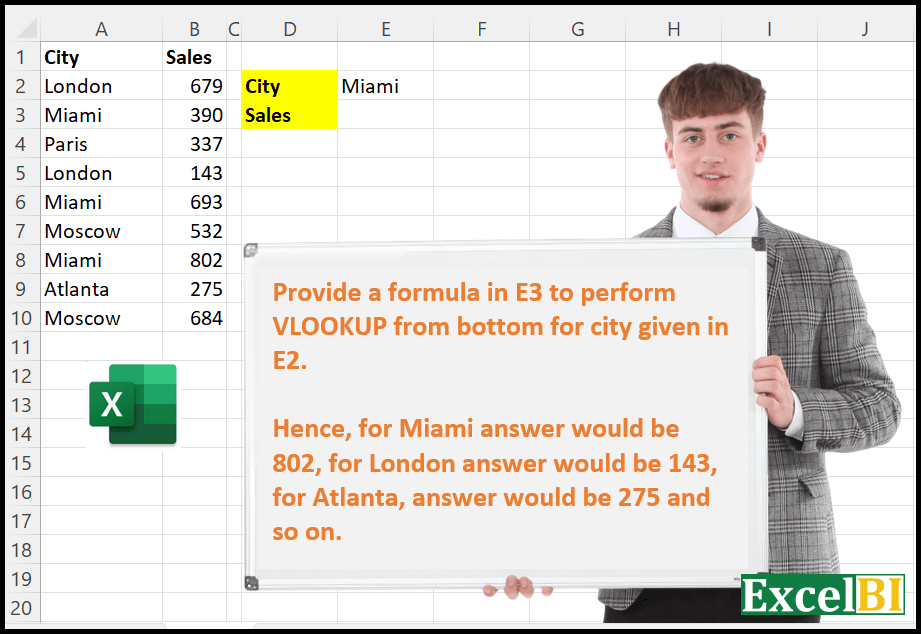
Provide a formula in E3 to perform VLOOKUP from bottom for city given in E2. Hence, for Miami answer would be 802, for London answer would be 143, for Atlanta, answer would be 275 and so on.
📌 Challenge Details and Links
ExcelBI Excel Challenge Number: 8
Challenge Difficulty: ⭐️
📥Download Sample File
📥Link to the solutions on LinkedIn
Solving the challenge of Bottom-Up VLOOKUP Formula with Power Query
Power Query solution 1 for Bottom-Up VLOOKUP Formula, proposed by Aditya Kumar Darak 🇮🇳:
let
  data     = Excel.CurrentWorkbook(){[Name = "data"]}[Content],
  criteria = Excel.CurrentWorkbook(){[Name = "criteria"]}[Content]{0}[City],
  Filter   = Table.SelectRows(data, each [City] = criteria)[Sales],
  Final    = List.Last(Filter)
in
  Final
Solving the challenge of Bottom-Up VLOOKUP Formula with Excel
Excel solution 1 for Bottom-Up VLOOKUP Formula, proposed by Rick Rothstein:
=INDEX(B:B,MAX(IF(A2:A10=E2,ROW(A2:A10))))Excel solution 2 for Bottom-Up VLOOKUP Formula, proposed by محمد حلمي:
=VLOOKUP(D3;SORT(A2:B10);2)Excel solution 3 for Bottom-Up VLOOKUP Formula, proposed by 🇰🇷 Taeyong Shin:
=--REGEXEXTRACT(CONCAT(A2:B10), ".*MiamiKd+")Excel solution 4 for Bottom-Up VLOOKUP Formula, proposed by 🇰🇷 Taeyong Shin:
=XLOOKUP(E2, A2:A10, B2:B10, , , -1)

Legacy
=VLOOKUP(1E5, B2:B10/(A2:A10=E2), 1, 1)
=INDEX(B2:B10, MATCH(0, B2:B10/(A2:A10=E2), -1))
=LOOKUP(1E5, B2:B10/(A2:A10=E2) )
=LOOKUP(1, 0/(A2:A10=E2), B2:B10)
Excel solution 5 for Bottom-Up VLOOKUP Formula, proposed by Julian Poeltl:
=XLOOKUP(E2,A2:A10,B2:B10,,,-1)
=VLOOKUP(E5,SORTBY(A2:B10,SEQUENCE(ROWS(A2:B10)),-1),2,FALSE)
Excel solution 6 for Bottom-Up VLOOKUP Formula, proposed by Timothée BLIOT:
=VLOOKUP(E2,SORTBY(A2:B10,SEQUENCE(ROWS(A2:A10)),-1),2,FALSE)Excel solution 7 for Bottom-Up VLOOKUP Formula, proposed by Bhavya Gupta:
=INDEX(B2:B10,MATCH(E2&MAXIFS(F2:F10,A2:A10,E2),A2:A10&F2:F10,0))Excel solution 8 for Bottom-Up VLOOKUP Formula, proposed by Bhavya Gupta:
=XLOOKUP(E2,A2:A10,B2:B10,,,-1)

=INDEX(B2:B10,XMATCH(E2,A2:A10,,-1))

=LOOKUP(2,1/(A2:A10=E2),B2:B10)
Excel solution 9 for Bottom-Up VLOOKUP Formula, proposed by Charles Roldan:
=LET(Flip, LAMBDA(f, f(f))(LAMBDA(f, LAMBDA(x, IF(ROWS(x) = 1, x, VSTACK(TAKE(x, -1), f(f)(DROP(x, -1))))))), VLOOKUP(E2, Flip(A2:B10), 2, 0))Excel solution 10 for Bottom-Up VLOOKUP Formula, proposed by 🇮🇷 Navid Esmaeilzadeh اسماعیل زاده:
=LOOKUP(2,1/($A$2:$A$10=E2),$B$2:$B$10)Excel solution 11 for Bottom-Up VLOOKUP Formula, proposed by Tolga Demirci, PMP, PMI-ACP, MOS-Expert:
=VLOOKUP(E2;INDEX(A1:B10;SORT(UNIQUE(IF(A2:B10<>"";ROW(A2:B10);"");FALSE);1;-1;FALSE);{12});2;0)Excel solution 12 for Bottom-Up VLOOKUP Formula, proposed by Jardiel Euflázio:
=VLOOKUP(

E2,
INDEX(A2:B10,SEQUENCE(ROWS(A2:B10),,ROWS(A2:B10),-1),{12}),
2,
0

)
Excel solution 13 for Bottom-Up VLOOKUP Formula, proposed by Jardiel Euflázio:
=INDIRECT("B"&MAX((A2:A10=E2)*ROW(A2:A10)))Excel solution 14 for Bottom-Up VLOOKUP Formula, proposed by Jardiel Euflázio:
=OFFSET(B1,MAX(IF(A2:A10=E2,SEQUENCE(ROWS(A2:A10)))),)Excel solution 15 for Bottom-Up VLOOKUP Formula, proposed by Jardiel Euflázio:
=LET(
    a,
    FILTER(
        B2:B10,
        A2:A10=E2
    ),
    INDEX(
        a,
        ROWS(
            a
        )
    )
)
Excel solution 16 for Bottom-Up VLOOKUP Formula, proposed by Jardiel Euflázio:
=XLOOKUP(E2,A2:A10,B2:B10,,,-1)Excel solution 17 for Bottom-Up VLOOKUP Formula, proposed by Jardiel Euflázio:
=TAKE(FILTER(B2:B10,A2:A10=E2),-1)Excel solution 18 for Bottom-Up VLOOKUP Formula, proposed by Sergei Baklan:
=VLOOKUP( 1E+33, 1/(A2:A10=E2)*B2:B10, 1, 1)Excel solution 19 for Bottom-Up VLOOKUP Formula, proposed by Cary Ballard, DML:
=VLOOKUP(E2, CHOOSEROWS(A2:B10, SEQUENCE(ROWS(A2:B10),,ROWS(A2:B10),-1)),2,0)Excel solution 20 for Bottom-Up VLOOKUP Formula, proposed by Juliano Santos Lima:
=LOOKUP(2,1/(A2:A10=E2),B2:B10)Excel solution 21 for Bottom-Up VLOOKUP Formula, proposed by Ibrahim Sadiq:
=LET(x,ROWS(A2:B10),VLOOKUP(E2,CHOOSEROWS(A2:B10,SEQUENCE(x,,x,-1)),2,0))Excel solution 22 for Bottom-Up VLOOKUP Formula, proposed by Nazmul Islam Jobair:
=VLOOKUP(
 E2,
 SORTBY(
 A2:B10,
 SEQUENCE(COUNTA(A2:A10)),
 -1
 ),
 2,
 FALSE
)
Excel solution 23 for Bottom-Up VLOOKUP Formula, proposed by John Gatonye:
=XLOOKUP($E$2,$A$2:$A$10,$B$2:$B$10,,0,-1)Excel solution 24 for Bottom-Up VLOOKUP Formula, proposed by Michael Szczesny:
=XLOOKUP(E21,$A$2:$A$10,$B$2:$B$10,,,-1)
 =MAX(IF($A$2:$A$10=$E$2,$B$2:$B$10,""))
Solving the challenge of Bottom-Up VLOOKUP Formula with Python in Excel
Python in Excel solution 1 for Bottom-Up VLOOKUP Formula, proposed by Alejandro Campos:
df = xl("A1:B10", headers=True)
lookup_value = xl("E2")
df_reversed = df.iloc[::-1]
result = df_reversed[df_reversed['City'] == lookup_value]['Sales'].iloc[0]
lookup_value, result
Python in Excel solution 2 for Bottom-Up VLOOKUP Formula, proposed by Aditya Kumar Darak 🇮🇳:
data = xl("A1:B10", True)
criteria = xl("E2")
result = data[data["City"] == criteria]["Sales"].iloc[-1]
result
&&&