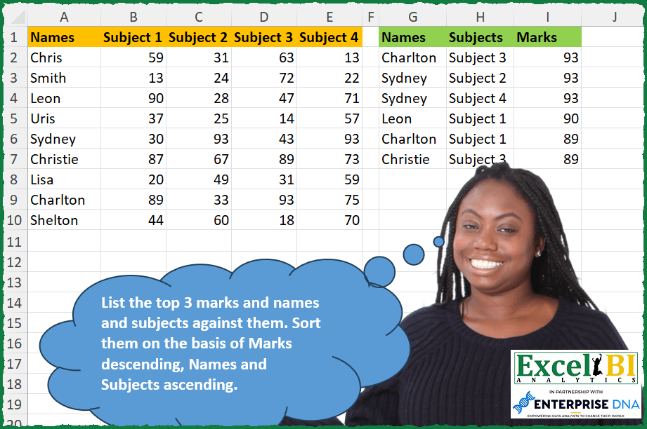
List the top 3 marks and names and subjects against them. Sort them on the basis of Marks descending, Names and Subjects ascending.
📌 Challenge Details and Links
ExcelBI Excel Challenge Number: 327
Challenge Difficulty: ⭐️
📥Download Sample File
📥Link to the solutions on LinkedIn
Solving the challenge of Top 3 marks with names and subjects with Power Query
Power Query solution 1 for Top 3 marks with names and subjects, proposed by Zoran Milokanović:
let
  Source = Table.Sort(
    Table.UnpivotOtherColumns(
      Excel.CurrentWorkbook(){[Name = "Input"]}[Content],
      {"Names"},
      "Subjects",
      "Marks"
    ),
    {{"Marks", 1}, "Names", "Subjects"}
  ),
  S = Table.SelectRows(
    Source,
    each List.PositionOf(List.FirstN(List.Distinct(Source[Marks]), 3), [Marks]) >= 0
  )
in
  S
Power Query solution 2 for Top 3 marks with names and subjects, proposed by Kris Jaganah:
let
  Source = Excel.CurrentWorkbook(){[Name = "Table1"]}[Content],
  Unpivot = Table.UnpivotOtherColumns(Source, {"Names"}, "Subjects", "Marks"),
  RankCol = Table.AddRankColumn(
    Unpivot,
    "Rank",
    {"Marks", Order.Descending},
    [RankKind = RankKind.Dense]
  ),
  Filter = Table.SelectRows(RankCol, each [Rank] <= 3),
  Sort = Table.Sort(
    Filter,
    {{"Marks", Order.Descending}, {"Names", Order.Ascending}, {"Subjects", Order.Ascending}}
  ),
  Remove = Table.RemoveColumns(Sort, {"Rank"})
in
  Remove
Power Query solution 3 for Top 3 marks with names and subjects, proposed by Alejandro Simón 🇵🇦 🇪🇸:
let
  Source = Excel.CurrentWorkbook(){[Name = "Table1"]}[Content],
  Group = Table.Group(
    Source,
    {"Names"},
    {
      {
        "All",
        each Table.FromColumns(
          List.Transform(Table.ToRows(Table.DemoteHeaders(_)), List.Skip),
          {"Subjects", "Marks"}
        )
      }
    }
  ),
  Expand = Table.ExpandTableColumn(Group, "All", Table.ColumnNames(Group[All]{0})),
  Sort = Table.Sort(Expand, {{"Marks", 1}, {"Names", 0}, {"Subjects", 0}}),
  Sol = Table.SelectRows(Sort, each [Marks] >= List.FirstN(List.Distinct(Sort[Marks]), 3){2})
in
  Sol
Power Query solution 4 for Top 3 marks with names and subjects, proposed by Alejandro Simón 🇵🇦 🇪🇸:
let
  Source  = Excel.CurrentWorkbook(){[Name = "Table1"]}[Content],
  Unpivot = Table.UnpivotOtherColumns(Source, {"Names"}, "Subjects", "Marks"),
  Sort    = Table.Sort(Unpivot, {{"Marks", 1}, {"Names", 0}, {"Subjects", 0}}),
  Sol     = Table.SelectRows(Sort, each [Marks] >= List.FirstN(List.Distinct(Sort[Marks]), 3){2})
in
  Sol
Power Query solution 5 for Top 3 marks with names and subjects, proposed by Luan Rodrigues:
let
  Fonte = Tabela1,
  col = Table.UnpivotOtherColumns(Fonte, {"Names"}, "Subjects", "Marks"),
  fil = Table.SelectRows(
    col,
    each List.ContainsAny({[Marks]}, List.MaxN(List.Distinct(col[Marks]), 3))
  ),
  res = Table.Sort(fil, {{each [Marks], 1}, {each [Names], 0}, {each [Subjects], 0}})
in
  res
Power Query solution 6 for Top 3 marks with names and subjects, proposed by Ramiro Ayala Chávez:
let
  Origen = Excel.CurrentWorkbook(){[Name = "Tabla1"]}[Content],
  a = Table.Group(
    Table.UnpivotOtherColumns(Origen, {"Names"}, "Subjects", "Marks"),
    {"Names"},
    {{"Group", each _}}
  )[[Group]],
  b = Table.Group(Table.Combine(a[Group]), {"Marks"}, {{"Group2", each _}}),
  c = Table.TransformColumns(
    Table.MaxN(b, "Marks", 3)[[Group2]],
    {"Group2", each Table.Sort(_, {{"Names", 0}, {"Subjects", 0}})}
  ),
  Sol = Table.Combine(c[Group2])
in
  Sol
Power Query solution 7 for Top 3 marks with names and subjects, proposed by Owen Price:
let
 Source = Excel.CurrentWorkbook(){[Name="t"]}[Content],
 unpivot = Table.Sort(Table.UnpivotOtherColumns(Source, {"Names"}, "Subjects", "Marks"),{{"Marks", Order.Descending}}) ,
 filt = Table.SelectRows(unpivot, each [Marks] >= List.Min(List.FirstN(List.Distinct(unpivot[Marks]),3)))
in
 filt


A Python option:

df = xl("t[hashtag#All]", headers=True).set_index("Names")
df = df.stack()
df = df.loc[df.isin(sorted(df.unique())[-3:])].reset_index()
df.columns = ['Names','Subjects','Marks']
df.sort_values(by=['Marks','Names','Subjects'],ascending=[False,True,True])
Power Query solution 8 for Top 3 marks with names and subjects, proposed by Rafael González B.:
let
  Source = Excel.CurrentWorkbook(){0}[Content],
  Din = Table.UnpivotOtherColumns(Source, {"Names"}, "Subjects", "Marks"),
  Rank = Table.AddRankColumn(
    Din,
    "Ranking",
    {"Marks", Order.Descending},
    [RankKind = RankKind.Dense]
  ),
  Max3 = Table.SelectRows(Rank, each ([Ranking] <= 3)),
  Sorting = Table.Sort(
    Max3,
    {{"Ranking", Order.Ascending}, {"Names", Order.Ascending}, {"Subjects", Order.Ascending}}
  ),
  FinalTab = Table.RemoveColumns(Sorting, {"Ranking"})
in
  FinalTab
Power Query solution 9 for Top 3 marks with names and subjects, proposed by Nicolas Micot:
let
 Source = Excel.CurrentWorkbook(){[Name="Tableau1"]}[Content],
 #"Type modifié" = Table.TransformColumnTypes(Source,{{"Names", type text}, {"Subject 1", Int64.Type}, {"Subject 2", Int64.Type}, {"Subject 3", Int64.Type}, {"Subject 4", Int64.Type}}),
 #"Tableau croisé dynamique des colonnes supprimé" = Table.UnpivotOtherColumns(#"Type modifié", {"Names"}, "Subject", "Mark"),
 #"Lignes triées" = Table.Sort(#"Tableau croisé dynamique des colonnes supprimé",{{"Mark", Order.Descending}}),
 #"Rang" = Table.AddRankColumn(#"Lignes triées", "rangMark", { "Mark", Order.Descending }, [ RankKind = RankKind.Dense ]),
 #"Lignes filtrées" = Table.SelectRows(Rang, each [rangMark] <= 3),
 #"Colonnes supprimées" = Table.RemoveColumns(#"Lignes filtrées",{"rangMark"})
in
 #"Colonnes supprimées"


        Show translation


        Show translation of this comment
Power Query solution 10 for Top 3 marks with names and subjects, proposed by Anup Kumar:
let
  Source = Excel.CurrentWorkbook(){[Name = "Table1"]}[Content],
  ChangedType = Table.TransformColumnTypes(
    Source,
    {
      {"Names", type text},
      {"Subject 1", Int64.Type},
      {"Subject 2", Int64.Type},
      {"Subject 3", Int64.Type},
      {"Subject 4", Int64.Type}
    }
  ),
  UnpivotedOtherColumns = Table.UnpivotOtherColumns(ChangedType, {"Names"}, "Subjects", "Marks"),
  AddedCustom = Table.AddRankColumn(
    UnpivotedOtherColumns,
    "Rank",
    {"Marks", Order.Descending},
    [RankKind = RankKind.Dense]
  ),
  FilteredRows = Table.SelectRows(AddedCustom, each [Rank] <= 3),
  RemovedColumns = Table.RemoveColumns(FilteredRows, {"Rank"}),
  #"Sorted Rows" = Table.Sort(
    RemovedColumns,
    {{"Marks", Order.Descending}, {"Names", Order.Ascending}, {"Subjects", Order.Ascending}}
  )
in
  #"Sorted Rows"
Power Query solution 11 for Top 3 marks with names and subjects, proposed by Ian Segard:
let
  Source = Excel.CurrentWorkbook(){[Name = "Table1"]}[Content],
  #"Changed Type" = Table.TransformColumnTypes(
    Source,
    {
      {"Names", type text},
      {"Subject 1", Int64.Type},
      {"Subject 2", Int64.Type},
      {"Subject 3", Int64.Type},
      {"Subject 4", Int64.Type}
    }
  ),
  #"Unpivoted Columns" = Table.UnpivotOtherColumns(#"Changed Type", {"Names"}, "Subject", "Grade"),
  #"Sorted Rows" = Table.Sort(
    #"Unpivoted Columns",
    {{"Grade", Order.Descending}, {"Names", Order.Ascending}, {"Subject", Order.Ascending}}
  ),
  #"Grouped Rows" = Table.Group(
    #"Sorted Rows",
    {"Grade"},
    {{"Count", each Table.RowCount(_), Int64.Type}}
  ),
  #"Sorted Rows1" = Table.Sort(#"Grouped Rows", {{"Grade", Order.Descending}}),
  #"Added Index" = Table.AddIndexColumn(#"Sorted Rows1", "Index", 1, 1, Int64.Type),
  Custom1 = #"Sorted Rows",
  #"Merged Queries" = Table.NestedJoin(
    Custom1,
    {"Grade"},
    #"Added Index",
    {"Grade"},
    "Custom1",
    JoinKind.LeftOuter
  ),
  #"Expanded Custom1" = Table.ExpandTableColumn(#"Merged Queries", "Custom1", {"Index"}, {"Index"}),
  #"Filtered Rows" = Table.SelectRows(#"Expanded Custom1", each [Index] <= 3),
  #"Removed Columns" = Table.RemoveColumns(#"Filtered Rows", {"Index"})
in
  #"Removed Columns"
Solving the challenge of Top 3 marks with names and subjects with Excel
Excel solution 1 for Top 3 marks with names and subjects, proposed by Bo Rydobon 🇹🇭:
=LET(
    p,
    B2:E10,
    m,
    TOCOL(
        p
    ),
    SORT(
        FILTER(
            HSTACK(
                TOCOL(
                    IF(
                        p,
                        A2:A10
                    )
                ),
                TOCOL(
                    IF(
                        p,
                        B1:E1
                    )
                ),
                m
            ),
            m>LARGE(
                UNIQUE(
                    m
                ),
                4
            )
        ),
        {3,
        1},
        {-1,
        1}
    )
)
Excel solution 2 for Top 3 marks with names and subjects, proposed by Rick Rothstein:
=SORT(
    TEXTSPLIT(
        TEXTJOIN(
            "*",
            ,
            TOCOL(
                LET(
                    a,
                    B2:F11,
                    m,
                    TAKE(
                        SORT(
                            UNIQUE(
                                TOCOL(
                                    a
                                )
                            ),
                            ,
                            -1
                        ),
                        3
                    ),
                    MAKEARRAY(
                        ROWS(
                                    a
                                ),
                        COLUMNS(
                                    a
                                ),
                        LAMBDA(
                            r,
                            c,
                            IF(
                                ISNUMBER(
                                    MATCH(
                                        INDEX(
                                            a,
                                            r,
                                            c
                                        ),
                                        m,
                                        0
                                    )
                                ),
                                INDEX(
                                    TAKE(
                                        OFFSET(
                                            a,
                                            0,
                                            -1
                                        ),
                                        ,
                                        1
                                    ),
                                    r
                                )&"|"&INDEX(
                                    TAKE(
                                        OFFSET(
                                            a,
                                            -1,

                                        ),
                                        1
                                    ),
                                    ,
                                    c
                                )&"|"&INDEX(
                                            a,
                                            r,
                                            c
                                        ),
                                1/0
                            )
                        )
                    )
                ),
                3
            )
        ),
        "|",
        "*"
    ),
    {3,
    1,
    2},
    {-1,
    1,
    1}
)
Excel solution 3 for Top 3 marks with names and subjects, proposed by John V.:
=LET(
    m,
    B2:E10,
    f,
    LAMBDA(
        x,
        TOCOL(
            IFS(
                m>LARGE(
                    UNIQUE(
                        TOCOL(
                            m
                        )
                    ),
                    4
                ),
                x
            ),
            2
        )
    ),
    SORT(
        HSTACK(
            f(
                A2:A10
            ),
            f(
                B1:E1
            ),
            f(
                            m
                        )
        ),
        {3;1},
        {-1;1}
    )
)
Excel solution 4 for Top 3 marks with names and subjects, proposed by محمد حلمي:
=LET(
    b,
    B2:E10,
    i,
    LAMBDA(
        v,
        TOCOL(
            IFS(
                b>LARGE(
                    UNIQUE(
                        TOCOL(
                            b
                        )
                    ),
                    4
                ),
                v
            ),
            2
        )
    ),
    SORT(
        HSTACK(
            i(
                A2:A10
            ),
            i(
                B1:E1
            ),
            i(
                            b
                        )
        ),
        {3,
        1},
        {-1,
        1}
    )
)
Excel solution 5 for Top 3 marks with names and subjects, proposed by 🇰🇷 Taeyong Shin:
=LET(d,TOCOL(B2:E10),tbl,TEXTSPLIT(CONCAT(A2:A10&", "&B1:E1&"|"),", ","|",1),SORT(GROUPBY(tbl,d,MAX,,0,,d>=LARGE(UNIQUE(d),3)),3,-1))Excel solution 6 for Top 3 marks with names and subjects, proposed by Kris Jaganah:
=LET(a,A2:A10,b,B2:E10,c,B1:E1,d,ROWS(a),e,COLUMNS(c),f,TOCOL(b),g,TOCOL(INDEX(c,SEQUENCE(e,d,,1/d)),,1),h,INDEX(a,SEQUENCE(d*e,,,1/e)),VSTACK({"Names","Subjects","Marks"},SORT(FILTER(HSTACK(h,g,f),LARGE(UNIQUE(f),3)<=f),{3,1,2},{-1,1,1})))Excel solution 7 for Top 3 marks with names and subjects, proposed by Kris Jaganah:
=LET(
    a,
    TOCOL(
        A2:A10&"-"&B1:E1&"#"&B2:E10
    ),
    b,
    TEXTBEFORE(
        a,
        "-"
    ),
    c,
    TEXTBEFORE(
        TEXTAFTER(
            a,
            "-"
        ),
        "#"
    ),
    d,
    --TEXTAFTER(
        a,
        "#"
    ),
    VSTACK(
        {"Names",
        "Subjects",
        "Marks"},
        SORT(
            FILTER(
                HSTACK(
                    b,
                    c,
                    d
                ),
                LARGE(
                    UNIQUE(
                        d
                    ),
                    3
                )<=d
            ),
            {3,
            1,
            2},
            {-1,
            1,
            1}
        )
    )
)
Excel solution 8 for Top 3 marks with &names and subjects, proposed by Julian Poeltl:
=LET(
    T,
    A1:E10,
    C,
    SORT(
        L_Flattena2DTableintoColumns(
            T
        ),
        3,
        -1
    ),
    M,
    LARGE(
        UNIQUE(
            CHOOSECOLS(
                C,
                3
            )
        ),
        3
    ),
    SORT(
        SORT(
            FILTER(
                C,
                CHOOSECOLS(
                C,
                3
            )>=M
            )
        ),
        3,
        -1
    )
)

Pre-programmed Lambdas:
L_Flattena2DTableintoColumns:
=LAMBDA(Table,
    LET(ROWS,
    ROWS(
        DROP(
            Table,
            1,
            1
        )
    ),
    COLUMNS,
    COLUMNS(
        DROP(
            Table,
            1,
            1
        )
    ),
    HRows,
    CHOOSEROWS(TAKE(
        Table,
        -ROWS,
        1
    ),
    (ROUNDDOWN(
        SEQUENCE(
            ROWS*COLUMNS,
            ,
            0
        )/COLUMNS,
        0
    )+1)),
    HColumn,
    CHOOSEROWS(
        TOCOL(
            TAKE(
                Table,
                1,
                -COLUMNS
            )
        ),
        L_RepeatingNumberSequence(
            COLUMNS,
            ROWS
        )
    ),
    Data,
    TOCOL(
        DROP(
            Table,
            1,
            1
        )
    ),
    HSTACK(
        HRows,
        HColumn,
        Data
    )))
L_RepeatingNumberSequence:
=LAMBDA(
    Numbers,
    Repetitions,
    IF(
        MOD(
            SEQUENCE(
                Numbers*Repetitions
            ),
            Numbers
        )=0,
        Numbers,
        MOD(
            SEQUENCE(
                Repetitions*Numbers
            ),
            Numbers
        )
    )
)
Excel solution 9 for Top 3 marks with names and subjects, proposed by Timothée BLIOT:
=LET(
    A,
    A2:A10,
    B,
    B1:E1,
    C,
    B2:E10,
    D,
    TOCOL(
        C
    ),
    SORT(
        FILTER(
            HSTACK(
                TOCOL(
                    IF(
                        A=C,
                        ,
                        A
                    )
                ),
                TOCOL(
                    IF(
                        B=C,
                        ,
                        B
                    )
                ),
                D
            ),
            D>=LARGE(
                UNIQUE(
                    D
                ),
                3
            )
        ),
        {3,
        1,
        2},
        {-1,
        1,
        1}
    )
)
Excel solution 10 for Top 3 marks with names and subjects, proposed by Hussein SATOUR:
=LET(
    v,
     B2:E10,
     a,
     TOCOL(
         A2:A10&"/"&B1:E1&"/"&v
     ),
     SORT(
         TEXTSPLIT(
             ARRAYTOTEXT(
                 FILTER(
                     a,
                      --TEXTAFTER(
                          a,
                           "/",
                           -1
                      )>LARGE(
                          UNIQUE(
                              TOCOL(
                                  v
                              )
                          ),
                           4
                      )
                 )
             ),
              "/",
              ", "
         ),
          {3,
         1,
         2},
         {-1,
         1,
         1}
     )
)
Excel solution 11 for Top 3 marks with names and subjects, proposed by Duy Tùng:
=LET(
    a,
    B2:E10,
    b,
    TOCOL(
        a
    ),
    SORT(
        GROUPBY(
            HSTACK(
                TOCOL(
                    IFS(
                        a,
                        A2:A10
                    )
                ),
                TOCOL(
                    IFS(
                        a,
                        B1:E1
                    )
                )
            ),
            b,
            SUM,
            ,
            0,
            ,
            b>LARGE(
                UNIQUE(
                    b
                ),
                4
            ),
            1
        ),
        3,
        -1
    )
)
hashtag#No2
=LET(
    a,
    B2:E10,
    f,
    LAMBDA(
        x,
        TOCOL(
            IF(
                MATCH(
                    a,
                    LARGE(
                        UNIQUE(
                            TOCOL(
        a
    )
                        ),
                        ROW(
                            1:3
                        )
                    ),

                ),
                x
            ),
            3
        )
    ),
    SORT(
        HSTACK(
            f(
                A2:A10
            ),
            f(
                B1:E1
            ),
            f(
        a
    )
        ),
        {3,
        1},
        {-1,
        1}
    )
)
Excel solution 12 for Top 3 marks with names and subjects, proposed by Sunny Baggu:
=LET(

     _marks,
     TAKE(
         UNIQUE(
             SORT(
                 BYROW(
                     B2:E10,
                      LAMBDA(
                          a,
                           MAX(
                               a
                           )
                      )
                 ),
                  ,
                  -1
             )
         ),
          3
     ),

     _r,
     REDUCE(

          {"Names",
          "Subjects",
          "Marks"},

          _marks,

          LAMBDA(
              a,
               v,

               IFNA(

                    VSTACK(

                         a,

                         HSTACK(
                             TOCOL(
                                 IF(
                                     B2:E10 = v,
                                      A2:A10,
                                      1 / x
                                 ),
                                  3
                             ),
                              TOCOL(
                                  IF(
                                      B2:E10 = v,
                                       B1:E1,
                                       1 / x
                                  ),
                                   3
                              ),
                              v
                         )

                    ),

                    v

               )

          )

     ),

     SORT(
         _r,
          {3,
          1},
          {-1,
          1}
     )

)
Excel solution 13 for Top 3 marks with names and subjects, proposed by Sunny Baggu:
=LET(

     _num,
     LARGE(
         UNIQUE(
             TOCOL(
                 B2:E10
             )
         ),
          3
     ),

     _col,
     TOCOL(

          HSTACK(

               IF(
                   B2:E10 >= _num,
                    A2:A10,
                    1 / x
               ),

               IF(
                   B2:E10 >= _num,
                    B1:E1,
                    1 / x
               ),

               IF(
                   B2:E10 >= _num,
                    B2:E10,
                    1 / x
               )

          ),

          3,

          1

     ),

     SORT(
         WRAPCOLS(
             _col,
              ROWS(
                  _col
              ) / 3
         ),
          {3,
          1},
          {-1,
          1}
     )

)
Excel solution 14 for Top 3 marks with names and subjects, proposed by LEONARD OCHEA 🇷🇴:
=LET(n,A2:A10,s,B1:E1,d,B2:E10,F,LAMBDA(x,TOCOL(IF(d,x,))),m,SORT(HSTACK(F(n),F(s),F(d)),{3,1},{-1,1}),FILTER(m,INDEX(m,,3)>LARGE(UNIQUE(F(d)) ,4)))Excel solution 15 for Top 3 marks with names and subjects, proposed by Abdallah Ally:
=LET(
    a,
    TOCOL(
        A2:A10&"-"&B1:E1
    ),
    b,
    HSTACK(
        TEXTBEFORE(
            a,
            "-"
        ),
        TEXTAFTER(
            a,
            "-"
        )
    ),
     c,
     TOCOL(
         B2:E10
     ),
     SORT(
         FILTER(
             HSTACK(
                 b,
                 c
             ),
              c>LARGE(
                  UNIQUE(
                      c
                  ),
                  4
              )
         ),
         {3,
         1,
         2},
         {-1,
         1,
         1}
     )
)
Excel solution 16 for Top 3 marks with names and subjects, proposed by Abdallah Ally:
=LET(
    a,
    DROP(
        REDUCE(
            "",
            TOCOL(
                A2:A10&"-"&B1:E1
            ),
             LAMBDA(
                 x,
                 y,
                 VSTACK(
                     x,
                     TEXTSPLIT(
                         y,
                         "-"
                     )
                 )
             )
        ),
        1
    ),
    b,
     TOCOL(
         B2:E10
     ),
     SORT(
         FILTER(
             HSTACK(
                 a,
                 b
             ),
             b>=LARGE(
                 UNIQUE(
                     b
                 ),
                 3
             )
         ),
         {3,
         1,
         2},
         {-1,
         1,
         1}
     )
)
Excel solution 17 for Top 3 marks with names and subjects, proposed by Bhavya Gupta:
=LET(
    s,
    TOCOL(
        IFNA(
            B1:E1,
            A2:A10
        )
    ),
    m,
    TOCOL(
        B2:E10
    ),
    n,
    TOCOL(
        IFNA(
            A2:A10,
            B1:E1
        )
    ),
    DROP(
        TAKE(
            GROUPBY(
                m,
                HSTACK(
                    n,
                    s,
                    m
                ),
                ARRAYTOTEXT,
                ,
                0,
                -1
            ),
            3
        ),
        ,
        1
    )
)
Excel solution 18 for Top 3 marks with names and subjects, proposed by Md. Zohurul Islam:
=LET(
    u,
    A2:A10,
    v,
    B1:E1,
    w,
    TOCOL(
        B2:E10
    ),

    hdr,
    {"Names",
    "Subjects",
    "Marks"},

    mx,
    TAKE(
        UNIQUE(
            SORT(
                w,
                ,
                -1
            )
        ),
        3
    ),

    a,
    HSTACK(
        TOCOL(
            IFNA(
                u,
                v
            )
        ),
        TOCOL(
            IFNA(
                v,
                u
            )
        ),
        w
    ),

    b,
    DROP(
        REDUCE(
            "",
            mx,
            LAMBDA(
                x,
                y,
                VSTACK(
                    x,
                    FILTER(
                        a,
                        w=y
                    )
                )
            )
        ),
        1
    ),

    d,
    SORT(
        b,
        {3,
        1,
        2},
        {-1,
        1,
        1}
    ),

    VSTACK(
        hdr,
        d
    )
)
Excel solution 19 for Top 3 marks with names and subjects, proposed by Asheesh Pahwa:
=LET(
    nm,
    B2:E10,
    t,
    TOCOL(
        nm
    ),
     u,
     UNIQUE(
         t
     ),

    I,
    LARGE(
        u{1;2;3}
    ),
    j,
    TOCOL(
        A2:A10&"-"&B1:E1&"-"&nm
    ),
    r,
    DROP(
        REDUCE(
            "",
            I,
            LAMBDA(
                x,
                y,
                VSTACK(
                    x,
                    LET(
                        a,
                        FIND(
                            y,
                            j
                        ),
                        b,
                        ISNUMBER(
                            a
                        ),
                        SORT(
                            FILTER(
                                j,
                                b
                            )
                        )
                    )
                )
            )
        ),
        1
    ),
    DROP(
        REDUCE(
            "",
            r,
            LAMBDA(
                a,
                v,
                VSTACK(
                    a,
                    TEXTSPLIT(
                        v,
                        "-"
                    )
                )
            )
        ),
        1
    )
)
Excel solution 20 for Top 3 marks with names and subjects, proposed by Pieter de Bruijn:
=LET(g,
    SORT(HSTACK(WRAPROWS(TOCOL(MAKEARRAY(ROWS(
        A2:A10
    ),
    8,
    LAMBDA(x,
    y,
    IF(ISODD(
        y
    ),
    INDEX(A2:A10,
    (x-1+(CEILING(
        y/8,
        1
    )))),
    INDEX(
        B1:E1,
        ,
        y/2
    ))))),
    2),
    TOCOL(
        B2:E10
    )),
    {3,
    1},
    {-1,
    1}),
    n,
    DROP(
        g,
        ,
        2
    ),
    FILTER(
        g,
        n>LARGE(
            UNIQUE(
                n
            ),
            4
        )
    ))

And looking at Taeyong Shin's solution I could've done:
=LET(
    n,
    TOCOL(
        B2:E10
    ),
    g,
    HSTACK(
        TEXTSPLIT(
            CONCAT(
                A2:A10&", "&B1:E1&"|"
            ),
            ", ",
            "|",
            1
        ),
        n
    ),
    SORT(
        FILTER(
        g,
        n>LARGE(
            UNIQUE(
                n
            ),
            4
        )
    ),
        {3,
        1},
        {-1,
        1}
    )
)
My first version has no restrictions to text length though (but that seems irrelevant in this situation)
Excel solution 21 for Top 3 marks with names and subjects, proposed by Ziad A.:
=SORTN(SPLIT(TOCOL(A2:A10&"|"&B1:E1&"|"&B2:E10),"|"),3,3,3,)Excel solution 22 for Top 3 marks with names and subjects, proposed by Giorgi Goderdzishvili:
=
LET(

    txt,
    A2:A10&"-"&B1:E1,

    tc,
    TOCOL(
        txt
    ),

    pt,
    TOCOL(
        B2:E10
    ),

    arr_,
     HSTACK(
         TEXTBEFORE(
             tc,
             "-"
         ),
          TEXTAFTER(
              tc,
              "-"
          )
     ),

    rnk,
     XMATCH(
         pt,
         UNIQUE(
             SORT(
                 pt,
                 ,
                 -1
             )
         )
     ),

    fn,
    SORT(
        FILTER(
            HSTACK(
                arr_,
                pt
            ),
            rnk<=3
        ),
        {3,
        1},
        {-1,
        1}
    ),

    fn
)
Excel solution 23 for Top 3 marks with names and subjects, proposed by Edwin Tisnado:
=LET(
    i,
    INDEX(
        SORT(
            UNIQUE(
                TOCOL(
                    B2:E10
                )
            ),
            ,
            -1
        ),
        3
    ),
    t,
    SORT(
        SORT(
            TEXTSPLIT(
                TEXTJOIN(
                    "/",
                    1,
                    TOCOL(
                        A2:A10&"*"&B1:E1&"*"&B2:E10
                    )
                ),
                "*",
                "/"
            ),
            1,
            1
        ),
        3,
        -1
    ),
    FILTER(
        t,
        --CHOOSECOLS(
            t,
            3
        )>=i
    )
)
Excel solution 24 for Top 3 marks with names and subjects, proposed by Andres Rojas Moncada:
=LET(ma,DIVIDIRTEXTO(UNIRCADENAS("*",1,A2:A10&"-"&B1:E1&"-"&B2:E10),"-","*"),ct,ELEGIRCOLS(ma,3)*1,ORDENAR(FILTRAR(ma,ct>=K.ESIMO.MAYOR(UNICOS(ct),3)),{3,1,2},{-1,1,1}))

English
=LET(ma,TEXTSPLIT(TEXTJOIN("*",1,A2:A10&"-"&B1:E1&"-"&B2:E10),"-","*"),ct,CHOOSECOLS(ma,3)*1,SORT(FILTER(ma,ct>=LARGE(UNIQUE(ct),3)),{3,1,2},{-1,1,1}))

English
=LET(ma,TEXTSPLIT(TEXTJOIN("*",1,A2:A10&"-"&B1:E1&"-"&B2:E10),"-","*"),ct,CHOOSECOLS(ma,3)*1,SORT(FILTER(IFERROR(ma*1,ma),ct>=LARGE(UNIQUE(ct),3)),{3,1,2},{-1,1,1}))
_x000D_
Excel solution 25 for Top 3 marks with names and subjects, proposed by Hazem Hassan:
=LET(
    a,
    B2:E10,
    SORT(
        TEXTSPLIT(
            CONCAT(
                TOCOL(
                    IF(
                        a>=LARGE(
                            TAKE(
                                SORT(
                                    UNIQUE(
                                        TOCOL(
                                            a
                                        )
                                    )
                                ),
                                -3
                            ),
                            3
                        ),
                        A2:A10&"-"&B1:E1&"-"&a,
                        1/0
                    ),
                    3
                )&"*"
            ),
            "-",
            "*",
            1
        ),
        {3,
        1},
        {-1,
        1}
    )
)
_x000D_
_x000D_
Excel solution 26 for Top 3 marks with names and subjects, proposed by Gabriel Raigosa:
=SORT(LET(d,B2:E10,e,TOCOL(d),x,TEXTSPLIT(TEXTJOIN("*",,A2:A10&"|"&B1:E1&"|"&d),"|","*"),FILTER(x,e>=LARGE(UNIQUE(e),3))),{3,1},{-1,1})

 ▶️ES:
=ORDENAR(LET(d,B2:E10,e,ENCOL(d),x,DIVIDIRTEXTO(UNIRCADENAS("*",,A2:A10&"|"&B1:E1&"|"&d),"|","*"),FILTRAR(x,e>=K.ESIMO.MAYOR(UNICOS(e),3))),{3,1},{-1,1})
_x000D_
_x000D_
Excel solution 27 for Top 3 marks with names and subjects, proposed by Sandro Barsonidze:
=LET(
a,SEQUENCE(COUNT(B2:E10)),

row_indx,  ROUNDUP(a/COUNTA(B1:E1),0),
col_indx,  MOD(a-1,COUNTA(B1:E1))+1,

names,  INDEX(A2:A10,row_indx),
subjects,  INDEX(B1:E1,col_indx),
marks,  INDEX(B2:E10,row_indx,col_indx),

table,  HSTACK(names,subjects,marks),

result,  SORT(FILTER(table,marks>=LARGE(UNIQUE(marks),3)),{3,1},{-1,1}),
result)
_x000D_
Solving the challenge of Top 3 marks with names and subjects with Python in Excel
_x000D_
Python in Excel solution 1 for Top 3 marks with names and subjects, proposed by John V.:
Hi everyone!
One [Python] option could be:
d = xl("A1:E10", headers = True).melt(h[0], var_name=h[1], value_name=h[2]).sort_values(by=[h[2], h[0]], ascending=[False, True])
d[d[h[2]] > d[h[2]].unique()[3]]
Blessings!
_x000D_
Solving the challenge of Top 3 marks with names and subjects with R
_x000D_
R solution 1 for Top 3 marks with names and subjects, proposed by Konrad Gryczan, PhD:
library(tidyverse)
library(readxl)
input = read_excel("Highest Marks Names Subjects.xlsx", range = "A1:E10")
test = read_excel("Highest Marks Names Subjects.xlsx", range = "G1:I7")
result = input %>%
 pivot_longer(-c(Names), names_to = "Subjects", values_to = "Marks") %>%
 mutate(rank = dense_rank(desc(Marks))) %>%
 filter(rank <= 3) %>%
 arrange(desc(Marks), Names, Subjects) %>%
 select(-rank)
_x000D_
_x000D_
R solution 2 for Top 3 marks with names and subjects, proposed by Krzysztof Nowak:
df <- read_xlsx("Highest Marks Names Subjects.xlsx",range = "A1:E10")
Matrix <- as.matrix(df[,2:ncol(df)])
Top3 <- unique(sort(as.vector(Matrix),decreasing = TRUE))[1:3]
Answer <- df |>
 pivot_longer(cols = 2:ncol(df),names_to = c("Subjects"),values_to = ("Marks")) |>
 filter(between(Marks,min(Top3),max(Top3))) |>
 arrange(desc(Marks), Names, Subjects)
Answer
_x000D_
&