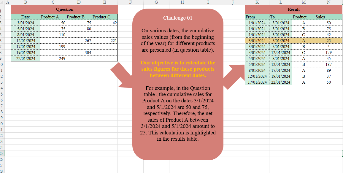
On various dates, the cumulative sales values (from the beginning of the year) for different products are presented (in the Question table). Our objective is to calculate the sales figures for these products between different dates. For example, in the Question table, the cumulative sales for Product A on the dates 3/1/2024 and 5/1/2024 are 50 and 75, respectively. Therefore, the net sales of Product A between 3/1/2024 and 5/1/2024 amount to 25. This calculation is highlighted in the results table.
📌 Challenge Details and Links
Challenge Number: 1
Challenge Difficulty: ⭐⭐⭐
📥Download Sample File
📥Link to the solutions on LinkedIn
Solving the challenge of Table Transformation! Part 1 with Power Query
Power Query solution 1 for Table Transformation! Part 1, proposed by Eric Laforce:
let
  Source = Table.TransformColumnTypes(
    Excel.CurrentWorkbook(){[Name = "rData"]}[Content],
    {{"Date", type date}}
  ),
  Prepare =
    let
      Unpivot = Table.UnpivotOtherColumns(Source, {"Date"}, "P", "S"),
      Filter  = Table.SelectRows(Unpivot, each ([S] <> ""))
    in
      Table.TransformColumns(Filter, {{"P", each Text.End(_, 1), type text}}),
  Transform =
    let
      Group = Table.Group(
        Prepare,
        {"P"},
        {
          "All",
          each List.Accumulate(
            Table.ToRows(_),
            [r = {}, p = {#date(2024, 1, 1), "", 0}],
            (s, c) => [r = s[r] & {{s[p]{0}, c{0}, c{1}, c{2} - s[p]{2}}}, p = c]
          )[r]
        }
      )
    in
      Table.FromRows(List.Combine(Group[All]), {"From", "To", "Product", "Sales"}),
  Sort = Table.Sort(Transform, {{"From", Order.Ascending}, {"Product", Order.Ascending}})
in
  Sort
Power Query solution 2 for Table Transformation! Part 1, proposed by Kris Jaganah:
let
  Source = Excel.CurrentWorkbook(){[Name = "Table1"]}[Content],
  Type = Table.TransformColumnTypes(
    Source,
    {
      {"Product A", Int64.Type},
      {"Product B", Int64.Type},
      {"Product C", Int64.Type},
      {"Date", type date}
    }
  ),
  Unpiv = Table.UnpivotOtherColumns(Type, {"Date"}, "Product", "Value"),
  Grup = Table.Group(Unpiv, {"Product"}, {{"All", each _}, {"Count", each Table.RowCount(_)}}),
  Index = Table.AddColumn(Grup, "Custom", each Table.AddIndexColumn([All], "Idx", [Count], - 1)),
  Xpan = Table.ExpandTableColumn(Index, "Custom", {"Date", "Value", "Idx"}, {"To", "Value", "Idx"}),
  Idx = Table.AddColumn(Xpan, "Idx-1", each [Idx] + 1),
  Merge = Table.NestedJoin(
    Idx,
    {"Product", "Idx-1"},
    Idx,
    {"Product", "Idx"},
    "Idx-1.1",
    JoinKind.LeftOuter
  ),
  Xpan1 = Table.ExpandTableColumn(Merge, "Idx-1.1", {"To", "Value"}, {"From", "Val"}),
  Sale = Table.AddColumn(Xpan1, "Sales", each [Value] - (if [Val] = null then 0 else [Val])),
  Jan = Table.TransformColumns(Sale, {"From", each if _ = null then #date(2024, 1, 1) else _}),
  Keep = Table.SelectColumns(Jan, {"From", "To", "Product", "Sales"}),
  Sort = Table.Sort(Keep, {{"From", Order.Ascending}, {"Product", Order.Ascending}}),
  S = Table.TransformColumns(Sort, {"Product", each Text.End(_, 1)})
in
  S
Power Query solution 3 for Table Transformation! Part 1, proposed by Mahmoud Bani Asadi:
let
  Source = Excel.CurrentWorkbook(){[Name = "Sales"]}[Content],
  Ch = Table.TransformColumnTypes(
    Source,
    {
      {"Product A", Int64.Type},
      {"Product B", Int64.Type},
      {"Product C", Int64.Type},
      {"Date", type date}
    }
  ),
  UnPiv = Table.UnpivotOtherColumns(Ch, {"Date"}, "Product", "Sale"),
  Gp = Table.Combine(
    Table.Group(
      UnPiv,
      {"Product"},
      {
        {
          "Tbl",
          each [
            a = Table.AddIndexColumn(_, "I", 0, 1),
            b = Table.AddColumn(
              a,
              "New",
              each [
                Sale = try [Sale] - a[Sale]{[I] - 1} otherwise [Sale],
                From = try a[Date]{[I] - 1} otherwise #date(Date.Year([Date]), 1, 1),
                To   = a[Date]{[I]}
              ]
            )
          ][b]
        }
      }
    )[Tbl]
  )[[Product], [New]],
  Ex2 = Table.ExpandRecordColumn(Gp, "New", {"Sale", "From", "To"}),
  SrtC = Table.SelectColumns(Ex2, {"From", "To", "Product", "Sale"}),
  Ch2 = Table.TransformColumnTypes(
    SrtC,
    {{"Product", type text}, {"Sale", Int64.Type}, {"From", type date}, {"To", type date}}
  ),
  SrtR = Table.Sort(Ch2, {{"From", Order.Ascending}, {"Product", Order.Ascending}})
in
  SrtR
Power Query solution 4 for Table Transformation! Part 1, proposed by 🇮🇷 Navid Esmaeilzadeh اسماعیل زاده:
let
  S = Excel.CurrentWorkbook(){[Name = "T"]}[Content],
  C = Table.TransformColumnTypes(
    S,
    {
      {"Date", type date},
      {"Product A", Int64.Type},
      {"Product B", Int64.Type},
      {"Product C", Int64.Type}
    }
  ),
  U = Table.UnpivotOtherColumns(C, {"Date"}, "Product", "Sale"),
  G = Table.Group(
    U,
    {"Product"},
    {{"Tbl", each _, type table [Date = nullable date, Product = text, Sale = number]}}
  ),
  MF = (TBL) =>
    let
      In = Table.AddIndexColumn(TBL, "I", 0, 1, Int64.Type),
      A1 = Table.AddColumn(In, "From", each try In[Date]{[I] - 1} otherwise "1/1/2024"),
      C1 = Table.TransformColumnTypes(A1, {{"From", type date}}),
      A2 = Table.AddColumn(C1, "Sales", each try [Sale] - C1[Sale]{[I] - 1} otherwise [Sale]),
      R2 = Table.SelectColumns(A2, {"From", "Date", "Product", "Sales"})
    in
      R2,
  I = Table.AddColumn(G, "MF", each MF([Tbl])),
  R = Table.SelectColumns(I, {"MF"}),
  E = Table.ExpandTableColumn(
    R,
    "MF",
    {"From", "Date", "Product", "Sales"},
    {"From", "Date", "Product", "Sales"}
  ),
  R2 = Table.RenameColumns(E, {{"Date", "To"}}),
  Sol = Table.Sort(R2, {{"From", Order.Ascending}, {"Product", Order.Ascending}})
in
  Sol
Power Query solution 5 for Table Transformation! Part 1, proposed by Bhavya Gupta:
let
  Source = Excel.CurrentWorkbook(){[Name = "Table1"]}[Content],
  ReplacedBlank = Table.ReplaceValue(
    Source,
    "",
    null,
    Replacer.ReplaceValue,
    List.Skip(Table.ColumnNames(Source))
  ),
  Unpivot = Table.UnpivotOtherColumns(ReplacedBlank, {"Date"}, "Product", "Sales"),
  Grouped = Table.Combine(
    Table.Group(
      Unpivot,
      {"Product"},
      {
        {
          "All",
          each Table.FromColumns(
            {
              {Date.StartOfMonth([Date]{0})} & List.RemoveLastN([Date]),
              [Date],
              [Product],
              List.Transform(List.Zip({[Sales], {0} & List.RemoveLastN([Sales])}), each _{0} - _{1})
            },
            {"From", "To", "Product", "Sales"}
          )
        }
      }
    )[All]
  ),
  Sorted = Table.Sort(Grouped, {{"From", Order.Ascending}})
in
  Sorted
Solving the challenge of Table Transformation! Part 1 with Excel
Excel solution 1 for Table Transformation! Part 1, proposed by Bo Rydobon 🇹🇭:
=SORT(DROP(REDUCE(0,C2:E2,LAMBDA(c,p,LET(a,N(XLOOKUP(p,C2:E2,+C3:E9)),b,FILTER(a,a),d,FILTER(B3:B9,a),VSTACK(c,DROP(CHOOSE({1,2,3,4},VSTACK(45292,d),d,p,b-VSTACK(0,b)),-1))))),1))Excel solution 2 for Table Transformation! Part 1, proposed by John Jairo Vergara Domínguez:
=SORT(
    DROP(
        REDUCE(
            0,
            C2:E2,
            LAMBDA(
                a,
                v,
                LET(
                    i,
                    TAKE(
                        v:E9,
                        ,
                        1
                    ),
                    d,
                    FILTER(
                        B2:B9,
                        i<""
                    ),
                    c,
                    FILTER(
                        i,
                        i<""
                    ),
                    VSTACK(
                        a,
                        HSTACK(
                            VSTACK(
                                45292,
                                DROP(
                                    d,
                                    -1
                                )
                            ),
                            d,
                            IF(
                                d,
                                RIGHT(
                                    v
                                )
                            ),
                            c-VSTACK(
                                0,
                                DROP(
                                    c,
                                    -1
                                )
                            )
                        )
                    )
                )
            )
        ),
        1
    )
)
Excel solution 3 for Table Transformation! Part 1, proposed by JvdV –:
=SORT(
    DROP(
        REDUCE(
            {0,
            0,
            0,
            0,
            0},
            C3:E9,
            LAMBDA(
                x,
                y,
                LET(
                    q,
                    INDEX(
                        C2:E2,
                        COLUMN(
                            y
                        )-2
                    ),
                    r,
                    INDEX(
                        x,
                        ,
                        3
                    ),
                    z,
                    r=q,
                    IF(
                        y,
                        VSTACK(
                            x,
                            HSTACK(
                                MAX(
                                    45292,
                                    INDEX(
                                        x,
                                        ,
                                        2
                                    )*z
                                ),
                                INDEX(
                                    B:B,
                                    ROW(
                            y
                        )
                                ),
                                q,
                                y-MAX(
                                    DROP(
                                        x,
                                        ,
                                        4
                                    )*z
                                ),
                                y
                            )
                        ),
                        x
                    )
                )
            )
        ),
        1,
        -1
    )
)

Assuming you don't really need to shorted product names. If so,
     add TEXTAFTER()
Excel solution 4 for Table Transformation! Part 1, proposed by Mahmoud Bani Asadi:
=LET(
    a,
     TOCOL(
         IFERROR(
             B3:B9,
              C2:E2
         )
     ),
     b,
     TOCOL(
         IFERROR(
             C2:E2,
              B3:B9
         )
     ),
     c,
     TOCOL(
         C3:E9
     ),
     d,
     HSTACK(
         a,
          b,
          c
     ),
     e,
     FILTER(
         d,
          TAKE(
              d,
               ,
               -1
          ) <> ""
     ),
     f,
     INDEX(
         e,
          ,
          1
     ),
     g,
     INDEX(
         e,
          ,
          2
     ),
     h,
     DROP(
         REDUCE(
             "",
              UNIQUE(
                  g
              ),
              LAMBDA(
                  x,
                  y,
                   VSTACK(
                       x,
                        LET(
                            m,
                             FILTER(
                                 e,
                                  g = y
                             ),
                             n,
                             TAKE(
                                 m,
                                  ,
                                  -1
                             ),
                             o,
                             IFERROR(
                                 n - VSTACK(
                                     "",
                                      DROP(
                                          n,
                                           -1
                                      )
                                 ),
                                  n
                             ),
                             p,
                             HSTACK(
                                 VSTACK(
                                     DATE(
                                         YEAR(
                                             INDEX(
                                                 m,
                                                  1,
                                                  1
                                             )
                                         ),
                                          1,
                                          1
                                     ),
                                      INDEX(
                                          DROP(
                                              m,
                                               -1
                                          ),
                                           ,
                                           1
                                      )
                                 ),
                                  DROP(
                                 m,
                                  ,
                                  -1
                             ),
                                  o
                             ),
                             p
                        )
                   )
              )
         ),
          1
     ),
     SORT(
         h
     )
)
Excel solution 5 for Table Transformation! Part 1, proposed by Sunny Baggu:
=LET(     _r,
     DROP(          REDUCE(

               "",

               C2:E2,

               LAMBDA(
                   a,
                    v,

                    VSTACK(

                         a,

                         LET(

                              _c,
                              FILTER(
                                  C3:E9,
                                   C2:E2 = v
                              ),

                              _c1,
                              FILTER(
                                  B3:B9,
                                   _c <> ""
                              ),

                              _c2,
                              VSTACK(
                                  DATE(
                                      2024,
                                       1,
                                       1
                                  ),
                                   DROP(
                                       _c1,
                                        -1
                                   )
                              ),

                              IFNA(
                                  HSTACK(
                                      _c2,
                                       _c1,
                                       v,
                                       XLOOKUP(
                                           _c1,
                                            B3:B9,
                                            _c
                                       ) - XLOOKUP(
                                           _c2,
                                            B3:B9,
                                            _c,
                                            0
                                       )
                                  ),
                                   v
                              )

                         )

                    )

               )

          ),          1     ),     SORT(
         _r
     ))
Excel solution 6 for Table Transformation! Part 1, proposed by Diego Pérez:
=LET(startdate,
    DATE(
        2024,
        1,
        1
    ),endofdays,
    DATE(
        2100,
        1,
        1
    ),rProd,
    DROP(
        Table2[        #Headers],
        ,
        1
    ),rValues,
    DROP(
        DROP(
            Table2[

            #All],
            1
        ),
        ,
        1
    ),rDates,
    Table2[Date],nProd,
    COUNTA(
        Table2[        #Headers]
    )-1,nDates,
    COUNTA(
        Table2[Date]
    ),unpArray,
     HSTACK(
 INDEX(rDates,
    1+(INT(
        SEQUENCE(
            nDates*nProd,
            1,
            0,
            1
        )/nProd
    ))), INDEX(rProd,
    MOD(SEQUENCE(
        nDates*nProd,
        1,
        0
    ),
    (nProd))+1), TOCOL(
     rValues
 )),janfirst,
    HSTACK(
        IF(
            SEQUENCE(
                COUNTA(
                    rProd
                ),
                1,
                1
            ),
            startdate
        ),
        TOCOL(
                    rProd
                ),
        SEQUENCE(
            nProd,
            1,
            0,
            0
        )
    ),declast,
    HSTACK(
        IF(
            SEQUENCE(
                COUNTA(
                    rProd
                ),
                1,
                1
            ),
            endofdays
        ),
        TOCOL(
                    rProd
                ),
        SEQUENCE(
            nProd,
            1,
            0,
            0
        )
    ),unparray2,
    SORT(
        VSTACK(
            janfirst,
            FILTER(
                unpArray,
                INDEX(
                    unpArray,
                    ,
                    3
                )>0
            ),
            declast
        ),
        2
    ),rangearray1,
    DROP(
        HSTACK(
            DROP(
                INDEX(
                    unparray2,
                    0,
                    1
                ),
                -1
            ),
            DROP(
                unparray2,
                1
            )
        ),
        ,
        -1
    ),lastdate,
    XLOOKUP(
        INDEX(
            rangearray1,
            0,
            2
        )&INDEX(
            rangearray1,
            0,
            3
        ),
        INDEX(
                    unparray2,
                    0,
                    1
                )&INDEX(
                    unparray2,
                    0,
                    2
                ),
        INDEX(
            unparray2,
            0,
            3
        ),
        0,
        0
    ),firstdate,
    XLOOKUP(
        INDEX(
            rangearray1,
            0,
            1
        )&INDEX(
            rangearray1,
            0,
            3
        ),
        INDEX(
                    unparray2,
                    0,
                    1
                )&INDEX(
                    unparray2,
                    0,
                    2
                ),
        INDEX(
            unparray2,
            0,
            3
        ),
        0,
        0
    ),vararray,
    SORT(
        HSTACK(
            rangearray1,
            lastdate-firstdate
        )
    ),FILTER(
    vararray,
    INDEX(
        vararray,
        ,
        4
    )>0
)
)
Excel solution 7 for Table Transformation! Part 1, proposed by Surendra Reddy:
=LET(a,C2:E2,b,C3:E9,d,B3:B9,MAP(L3:L13,M3:M13,K3:K13,LAMBDA(x,y,z,XLOOKUP(x,d,XLOOKUP(y,RIGHT(a),b))-XLOOKUP(z,d,XLOOKUP(y,RIGHT(a),b),0))))Excel solution 8 for Table Transformation! Part 1, proposed by Surendra Reddy:
=LET(
    a,
    C2:E2,
    b,
    C3:E9,
    d,
    B3:B9,
    MAP(
        L3:L13,
        M3:M13,
        K3:K13,
        LAMBDA(
            x,
            y,
            z,
            XLOOKUP(
                x,
                d,
                INDEX(
                    b,
                    ,
                    XMATCH(
                        y,
                        RIGHT(
                            a
                        )
                    )
                ),
                0
            )-XLOOKUP(
                z,
                d,
                INDEX(
                    b,
                    ,
                    XMATCH(
                        y,
                        RIGHT(
                            a
                        )
                    )
                ),
                0
            )
        )
    )
)
Excel solution 9 for Table Transformation! Part 1, proposed by Surendra Reddy:
=LET(
    a,
    C2:E2,
    b,
    C3:E9,
    d,
    B3:B9,
    MAP(
        L3:L13,
        M3:M13,
        K3:K13,
        LAMBDA(
            x,
            y,
            z,
            IFERROR(
                INDEX(
                    b,
                    XMATCH(
                        x,
                        d
                    ),
                    XMATCH(
                        y,
                        RIGHT(
                            a
                        )
                    )
                ),
                0
            )-IFERROR(
                INDEX(
                    b,
                    XMATCH(
                        z,
                        d
                    ),
                    XMATCH(
                        y,
                        RIGHT(
                            a
                        )
                    )
                ),
                0
            )
        )
    )
)
Excel solution 10 for Table Transformation! Part 1, proposed by Surendra Reddy:
=LET(
    a,
    C2:E2,
    b,
    C3:E9,
    d,
    B3:B9,
    MAP(
        L3:L13,
        M3:M13,
        K3:K13,
        LAMBDA(
            x,
            y,
            z,
            XLOOKUP(
                x,
                d,
                CHOOSECOLS(
                    b,
                    XMATCH(
                        y,
                        RIGHT(
                            a
                        )
                    )
                ),
                0
            )-XLOOKUP(
                z,
                d,
                CHOOSECOLS(
                    b,
                    XMATCH(
                        y,
                        RIGHT(
                            a
                        )
                    )
                ),
                0
            )
        )
    )
)
Excel solution 11 for Table Transformation! Part 1, proposed by Surendra Reddy:
=LET(
    a,
    C2:E2,
    b,
    C3:E9,
    d,
    B3:B9,
    MAP(
        L3:L13,
        M3:M13,
        K3:K13,
        LAMBDA(
            x,
            y,
            z,
            IFERROR(
                CHOOSECOLS(
                    CHOOSEROWS(
                        b,
                        XMATCH(
                            x,
                            d
                        )
                    ),
                    XMATCH(
                        y,
                        RIGHT(
                            a
                        )
                    )
                ),
                0
            )-IFERROR(
                CHOOSECOLS(
                    CHOOSEROWS(
                        b,
                        XMATCH(
                            z,
                            d
                        )
                    ),
                    XMATCH(
                        y,
                        RIGHT(
                            a
                        )
                    )
                ),
                0
            )
        )
    )
)