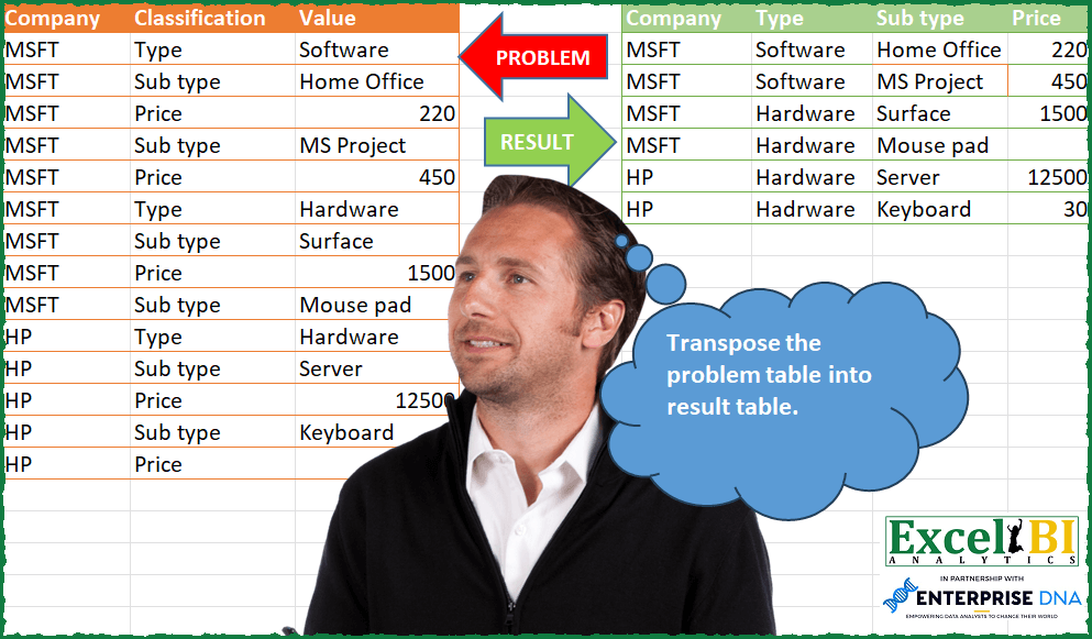
Transpose the problem table into result table.
📌 Challenge Details and Links
ExcelBI Power Query Challenge Number: 84
Challenge Difficulty: ⭐️⭐️⭐️⭐️⭐️⭐️
📥Download Sample File
📥Link to the solutions on LinkedIn
Solving the challenge of Transpose to Desired Table Format with Power Query
Power Query solution 1 for Transpose to Desired Table Format, proposed by Bo Rydobon 🇹🇭:
let
  Source = Excel.CurrentWorkbook(){[Name = "Table1"]}[Content],
  Group = Table.Combine(
    Table.Group(
      Source,
      "Classification",
      {"T", each Table.Pivot(_, List.Distinct([Classification]), "Classification", "Value")},
      0,
      (b, e) => Number.From(Text.Contains(e, "ype"))
    )[T]
  ),
  Ans = Table.SelectRows(Table.FillDown(Group, {"Type"}), each [#"Sub type"] <> null)
in
  Ans
Power Query solution 2 for Transpose to Desired Table Format, proposed by Zoran Milokanović:
let
  Source = Excel.CurrentWorkbook(){[Name = "Input"]}[Content],
  AdjustTable = Table.FromRows(
    List.Accumulate(
      Table.ToRows(Source),
      {},
      (s, c) =>
        s
          & (
            if c{1} = "Sub type" and (List.Last(s){1}? ?? "") <> "Type" then
              {List.Last(List.Select(s, each _{1} = "Type"))}
            else
              {}
          )
          & {c}
    ),
    Table.ColumnNames(Source)
  ),
  AddIndex = Table.ExpandTableColumn(
    Table.Group(
      AdjustTable,
      {"Company", "Classification"},
      {{"Data", each Table.AddIndexColumn(_, "Index")}}
    )[[Data]],
    "Data",
    {"Company", "Classification", "Value", "Index"}
  ),
  Solution = Table.Sort(
    Table.RemoveColumns(
      Table.Pivot(AddIndex, List.Distinct(AddIndex[Classification]), "Classification", "Value"),
      {"Index"}
    ),
    {
      {each List.PositionOf(List.Distinct(Source[Company]), [Company]), 0},
      {
        each List.PositionOf(
          List.Distinct(Table.SelectRows(Source, each ([Classification] = "Type"))[Value]),
          [Type]
        ),
        0
      },
      {
        each List.PositionOf(
          List.Distinct(Table.SelectRows(Source, each ([Classification] = "Sub type"))[Value]),
          [Sub type]
        ),
        0
      }
    }
  )
in
  Solution
Power Query solution 3 for Transpose to Desired Table Format, proposed by Kris Jaganah:
let
  Source = Excel.CurrentWorkbook(){[Name = "Table1"]}[Content],
  Indx   = Table.AddIndexColumn(Source, "Index", 1, 1, Int64.Type),
  Pivot  = Table.Pivot(Indx, List.Distinct(Indx[Classification]), "Classification", "Value"),
  Down   = Table.FillDown(Pivot, {"Type"}),
  Up     = Table.FillUp(Down, {"Price"}),
  Filter = Table.SelectRows(Up, each ([Sub type] <> null)),
  Sort   = Table.Sort(Filter, {{"Index", Order.Ascending}}),
  Remove = Table.RemoveColumns(Sort, {"Index"})
in
  Remove
Power Query solution 4 for Transpose to Desired Table Format, proposed by Alejandro Simón 🇵🇦 🇪🇸:
let
  Source = Excel.CurrentWorkbook(){[Name = "Table1"]}[Content],
  Type = Table.AddColumn(Source, "Type", each if [Classification] = "Type" then [Value] else null),
  Prod = Table.AddColumn(
    Type,
    "Prod",
    each if Value.Type([Value]) = type number then null else [Value]
  ),
  Fill = Table.SelectRows(Table.FillDown(Prod, {"Prod", "Type"}), each ([Classification] <> "Type")),
  Sol = Table.Sort(
    Table.RemoveColumns(
      Table.Pivot(Fill, List.Distinct(Fill[Classification]), "Classification", "Value"),
      "Prod"
    ),
    each List.PositionOf(List.Distinct(Fill[Prod]), [Sub type])
  )
in
  Sol
Power Query solution 5 for Transpose to Desired Table Format, proposed by Alejandro Simón 🇵🇦 🇪🇸:
let
  Source = Excel.CurrentWorkbook(){[Name = "Table1"]}[Content],
  Type = Table.AddColumn(Source, "Type", each if [Classification] = "Type" then [Value] else null),
  Prod = Table.AddColumn(
    Type,
    "Prod",
    each if Value.Type([Value]) = type number then null else [Value]
  ),
  Fill = Table.SelectRows(Table.FillDown(Prod, {"Prod", "Type"}), each ([Classification] <> "Type")),
  Group = Table.Group(
    Fill,
    {"Company", "Type"},
    {
      {
        "Count",
        each
          let
            a = _,
            b = Table.RemoveColumns(a, {"Company", "Type"}),
            c = Table.RemoveColumns(
              Table.Pivot(b, List.Distinct([Classification]), "Classification", "Value"),
              "Prod"
            ),
            d = Table.Sort(c, each List.PositionOf(List.Distinct(b[Prod]), [#"Sub type"]))
          in
            d
      }
    }
  ),
  Sol = Table.ExpandTableColumn(Group, "Count", {"Sub type", "Price"})
in
  Sol
Power Query solution 6 for Transpose to Desired Table Format, proposed by Luan Rodrigues:
let
  Fonte = Tabela1,
  ind = Table.AddIndexColumn(Fonte, "Índice", 1, 1, Int64.Type),
  pb = Table.Pivot(ind, List.Distinct(ind[Classification]), "Classification", "Value"),
  pa = Table.FillDown(pb, {"Type"}),
  gp = Table.Group(
    pa,
    {"Company", "Type"},
    {
      {
        "Contagem",
        each Table.Distinct(
          Table.FillUp(
            Table.SelectRows(Table.FillDown(_, {"Sub type"}), each [Sub type] <> null),
            {"Price"}
          ),
          {"Company", "Sub type", "Price"}
        )
      }
    }
  ),
  rs = Table.RemoveColumns(
    Table.Sort(
      Table.ExpandTableColumn(gp, "Contagem", {"Sub type", "Price", "Índice"}),
      {{"Índice", Order.Ascending}}
    ),
    {"Índice"}
  )
in
  rs
Power Query solution 7 for Transpose to Desired Table Format, proposed by Brian Julius:
let
  Source = Excel.CurrentWorkbook(){[Name = "Table1"]}[Content],
  AddType = Table.SelectRows(
    Table.FillDown(
      Table.AddColumn(Source, "Type", each if [Classification] = "Type" then [Value] else null),
      {"Type"}
    ),
    each [Classification] <> "Type"
  ),
  AddSubType = Table.FillDown(
    Table.AddColumn(
      AddType,
      "SubType",
      each if [Classification] = "Sub type" then [Value] else null
    ),
    {"SubType"}
  ),
  PriceTable = Table.PrefixColumns(
    Table.SelectRows(AddSubType, each [Classification] = "Price"),
    "P"
  ),
  Join = Table.RemoveColumns(
    Table.Join(
      AddSubType,
      {"Company", "SubType"},
      PriceTable,
      {"P.Company", "P.SubType"},
      JoinKind.LeftOuter
    ),
    {"P.Company", "P.Classification", "P.Type", "P.SubType"}
  ),
  Clean = Table.RemoveColumns(
    Table.RenameColumns(
      Table.SelectRows(Join, each [Classification] <> "Price"),
      {"P.Value", "Price"}
    ),
    {"Classification", "Value"}
  )
in
  Clean
Power Query solution 8 for Transpose to Desired Table Format, proposed by Eric Laforce:
let
  Source = Excel.CurrentWorkbook(){[Name = "tData84"]}[Content],
  Transform = List.Accumulate(
    {"Type", "Sub type"},
    Source,
    (s, c) =>
      let
        _AddCol = Table.AddColumn(s, c, each if [Classification] = c then [Value] else null)
      in
        Table.FillDown(_AddCol, {c})
  ),
  FilterRows = Table.SelectRows(Transform, each ([Classification] <> "Type")),
  Group = Table.Group(
    FilterRows,
    {"Company", "Type", "Sub type"},
    {
      "Price",
      each try Table.SelectRows(_, each ([Classification] = "Price"))[Value]{0} otherwise null
    }
  )
in
  Group
Power Query solution 9 for Transpose to Desired Table Format, proposed by Victor Wang:
let
  Source = Excel.CurrentWorkbook(){[Name = "Table1"]}[Content],
  addType = Table.AddColumn(
    Source,
    "Type",
    each if [Classification] = "Type" then [Value] else null
  ),
  fillType = Table.FillDown(addType, {"Type"}),
  filterClass = Table.SelectRows(fillType, each ([Classification] <> "Type")),
  getRecords = Table.Group(
    filterClass,
    {"Company", "Type", "Classification"},
    {{"all", each Record.FromList([Value], [Classification])}},
    GroupKind.Local,
    (firstRecord, secondRecord) => Number.From(secondRecord[Classification] = "Sub type")
  ),
  expandRecord = Table.ExpandRecordColumn(getRecords, "all", {"Sub type", "Price"}),
  removeClass = Table.RemoveColumns(expandRecord, {"Classification"})
in
  removeClass
Solving the challenge of Transpose to Desired Table Format with Excel
Excel solution 1 for Transpose to Desired Table Format, proposed by Bo Rydobon 🇹🇭:
=LET(z,A2:C15,b,INDEX(z,,2),r,SEQUENCE(ROWS(z)),s,FILTER(r,LEFT(b)="S"),VSTACK(HSTACK(A1,TOROW(UNIQUE(b))),HSTACK(INDEX(z,HSTACK(s,LOOKUP(s,r/(b="type")),s),{1,3,3}),IFERROR(--INDEX(z,s+1,3),""))))Excel solution 2 for Transpose to Desired Table Format, proposed by Sunny Baggu:
=LET(_rows,SEQUENCE(ROWS(A2:A15)),_uclass,UNIQUE(B2:B15),_cnt,MAP(_uclass,LAMBDA(a,ROWS(FILTER(B2:B15,B2:B15=a)))),_classmax,FILTER(_uclass,_cnt=MAX(_cnt)),_subtypenum,FILTER(_rows,B2:B15=_classmax),_comp,INDEX(A2:A15,_subtypenum),_typnum,FILTER(_rows,B2:B15="Type"),_typnumlist,XLOOKUP(_subtypenum,_typnum,_typnum,,-1),_type,INDEX(C2:C15,_typnumlist),_subtype,INDEX(C2:C15,_subtypenum),_pricenum,FILTER(_rows,B2:B15="Price"),_pricenumlist,XLOOKUP(_subtypenum+1,_pricenum,_pricenum),_price,IFNA(INDEX(C2:C15,_pricenumlist),""),HSTACK(_comp,_type,_subtype,_price))Solving the challenge of Transpose to Desired Table Format with Excel VBA
Excel VBA solution 1 for Transpose to Desired Table Format, proposed by محمد حلمي:
=LET(b,B2:B15,c,C2:C15,r,FILTER(c,b="Sub type"),v,
XMATCH(r,c),u,INDEX(c,v-1),VSTACK(HSTACK(A1,
TOROW(UNIQUE(b))),HSTACK(INDEX(A2:A15,v),IF(u>"@",u,VSTACK(0,DROP(u,-1))),r,IFERROR(--INDEX(c,v+1),""))))
Excel VBA solution 2 for Transpose to Desired Table Format, proposed by محمد حلمي:
=LET(b,B2:B15,c,C2:C15,r,FILTER(c,b="Sub type"),v,
XMATCH(r,c),l,INDEX(c,v+1),u,INDEX(c,v-1),VSTACK(
HSTACK(A1,TOROW(UNIQUE(b))),HSTACK(INDEX(A2:A15,v),IF(ISTEXT(u),u,VSTACK(0,DROP(u,-1))),r,IF(ISTEXT(l),"",l))))
Excel VBA solution 3 for Transpose to Desired Table Format, proposed by Oscar Mendez Roca Farell:
=LET(_a, A2:A15,_b, B2:B15,_c, C2:C15,_m, MAP(_b,_c, LAMBDA(b,c,LOOKUP(2, 1/(B2:b="Type"), C2:c))),_r, REDUCE(TOROW(DROP(UNIQUE(_b), 1)), UNIQUE(_a), LAMBDA(i,x, VSTACK(i, WRAPROWS(FILTER(_c, (_b<>"Type")*(_a=x)), 2, "")))), HSTACK(VSTACK(HSTACK(A1,"Type"), FILTER(HSTACK(_a,_m),_b="Sub type")),_r))
Excel VBA solution 4 for Transpose to Desired Table Format, proposed by Tolga Demirci, PMP, PMI-ACP, MOS-Expert:
=LET(e;FILTER(C2:C15;B2:B15="Sub type");VSTACK(HSTACK("Company";TOROW(UNIQUE(B2:B15)));HSTACK(e;LET(y;LET(x;IF(ISNUMBER(MAP(B2:B15;LAMBDA(a;MATCH("Type";a;0))));ROW(INDIRECT("A2:"&"A"&COUNTA(A2:A15)));"");FILTER(x;x<>""));INDEX(C2:C15;MAP(XMATCH(e;C2:C15;0)+1;LAMBDA(b;MAX(FILTER(y;b>y))-1))));e;LET(c;INDEX(C2:C15;XMATCH(e;C2:C15;0)+1);IF(ISNUMBER(c);c;"")))))
&&&