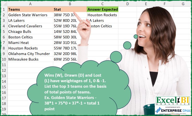
Wins (W), Drawn (D) and Lost (L) have weightages of 1, 0 & -1. List the top 3 teams on the basis of total points of teams. Ex. Golden State Warriors – 38*1 + 75*0 + 37*-1 = total 1 point
📌 Challenge Details and Links
ExcelBI Excel Challenge Number: 304
Challenge Difficulty: ⭐️
📥Download Sample File
📥Link to the solutions on LinkedIn
Solving the challenge of Rank Teams by Total Points with Power Query
Power Query solution 1 for Rank Teams by Total Points, proposed by Bo Rydobon 🇹🇭:
let
  Source = Excel.CurrentWorkbook(){[Name = "Table1"]}[Content],
  Win = Table.AddColumn(
    Source,
    "W",
    each
      let
        t = Text.SplitAny([Stat], "WDL ")
      in
        Expression.Evaluate(t{0} & "-" & t{4})
  ),
  Ans = Table.Sort(
    Table.SelectRows(Win, each [W] >= List.Last(List.MaxN(List.Distinct(Win[W]), 3))),
    each - [W]
  )[[Teams]]
in
  Ans
Power Query solution 2 for Rank Teams by Total Points, proposed by Zoran Milokanović:
let
  Source = Excel.CurrentWorkbook(){[Name = "Input"]}[Content],
  P = Table.Sort(
    Table.AddColumn(
      Source,
      "W",
      each Expression.Evaluate(
        List.Accumulate(
          {{"W", "*1"}, {"D", "*0"}, {"L", "*-1"}, {" ", "+"}},
          [Stat],
          (s, c) => Text.Replace(s, c{0}, c{1})
        )
      )
    ),
    {"W", 1}
  ),
  S = Table.FirstN(
    P,
    each List.Count(List.Distinct(List.FirstN(P[W], List.PositionOf(P[W], [W]) + 1))) < 4
  )[Teams]
in
  S
Power Query solution 3 for Rank Teams by Total Points, proposed by Aditya Kumar Darak 🇮🇳:
let
  Source = Excel.CurrentWorkbook(){[Name = "dara"]}[Content],
  Return = Table.MaxN(
    Source,
    each [S = Text.SplitAny([Stat], " WDL"), T = Number.From(S{0}) - Number.From(S{4})][T],
    3
  )[Teams]
in
  Return
Power Query solution 4 for Rank Teams by Total Points, proposed by Alejandro Simón 🇵🇦 🇪🇸:
let
  Source = Excel.CurrentWorkbook(){[Name = "Table1"]}[Content],
  Sol = Table.MaxN(
    Table.Sort(
      Table.AddColumn(
        Source,
        "Custom",
        each
          let
            a = Text.Split([Stat], " "),
            b = List.Transform(a, each Number.From(Text.Remove(_, {"A" .. "Z"}))),
            c = b{0} - b{2}
          in
            c
      ),
      {"Custom", 1}
    ),
    "Custom",
    3
  )[[Teams]]
in
  Sol
Power Query solution 5 for Rank Teams by Total Points, proposed by Luan Rodrigues:
let
  Fonte = Tabela1,
  trf = Table.TransformColumns(
    Fonte,
    {
      {
        "Stat",
        each Expression.Evaluate(
          Text.Combine(
            List.Select(
              List.ReplaceMatchingItems(
                Text.ToList(_),
                List.Zip({{"W", "D", "L"}, {"*1+", "*0+", "*-1"}})
              ),
              each _ <> " "
            )
          )
        ),
        type number
      }
    }
  ),
  res = Table.Sort(
    Table.SelectRows(trf, each List.ContainsAny({[Stat]}, List.MaxN(trf[Stat], 3))),
    {"Stat", 1}
  )[Teams]
in
  res
Power Query solution 6 for Rank Teams by Total Points, proposed by Ramiro Ayala Chávez:
let
  Origen = Excel.CurrentWorkbook(){[Name = "Tabla1"]}[Content],
  a = Table.RemoveColumns(
    Table.SplitColumn(
      Origen,
      "Stat",
      Splitter.SplitTextByDelimiter(" ", QuoteStyle.Csv),
      {"W", "D", "L"}
    ),
    "D"
  ),
  b = Table.SplitColumn(
    a,
    "W",
    Splitter.SplitTextByCharacterTransition({"0" .. "9"}, {"W"}),
    {"W1", "W2"}
  ),
  c = Table.SplitColumn(
    b,
    "L",
    Splitter.SplitTextByCharacterTransition({"0" .. "9"}, {"L"}),
    {"L1", "L2"}
  ),
  d = Table.TransformColumnTypes(c, {{"W1", Int64.Type}, {"L1", Int64.Type}}),
  e = Table.AddColumn(d, "Points", each [W1] - [L1])[[Teams], [Points]],
  Sol = Table.RenameColumns(
    Table.FirstN(Table.Sort(e, {{"Points", 1}}), 3)[[Teams]],
    {{"Teams", "Answer Expected"}}
  )
in
  Sol
Power Query solution 7 for Rank Teams by Total Points, proposed by Rafael González B.:
let
  Source = Excel.CurrentWorkbook(){0}[Content],
  Pt = Table.AddColumn(
    Source,
    "Points",
    each
      let
        a = [Stat],
        b = Text.Split(a, " "),
        c = List.Transform(b, each Number.From(Text.Remove(_, {"A" .. "Z"}))),
        d = (c{0} * 1) + (c{1} * 0) + (c{2} * - 1)
      in
        d
  ),
  Rank = Table.AddRankColumn(Pt, "Rank", {"Points", Order.Descending}, [RankKind = 1]),
  Anw = Table.SelectRows(Rank, each [Rank] <= 3)[[Teams]]
in
  Anw
Power Query solution 8 for Rank Teams by Total Points, proposed by Luke Jarych:
let
  Source = Table1,
  W = "*1",
  D = "*0",
  L = "*-1",
  #"Replaced Value" = Table.ReplaceValue(Source, " ", "+", Replacer.ReplaceText, {"Stat"}),
  #"Added Custom1" = Table.AddColumn(
    #"Replaced Value",
    "Custom",
    each Text.Replace(Text.Replace(Text.Replace([Stat], "W", W), "D", D), "L", L)
  ),
  #"Added Custom2" = Table.AddColumn(
    #"Added Custom1",
    "Custom.1",
    each Expression.Evaluate([Custom])
  ),
  SortedTable = Table.Sort(#"Added Custom2", {{"Custom.1", Order.Descending}}),
  Top3Results = Table.FirstN(SortedTable, 3),
  #"Removed Other Columns" = Table.SelectColumns(Top3Results, {"Teams"})
in
  #"Removed Other Columns"
Power Query solution 9 for Rank Teams by Total Points, proposed by Alejandra Horvath CPA, CGA:
let
  Source = Excel.CurrentWorkbook(){[Name = "Table1"]}[Content],
  TfrCol = Table.TransformColumns(
    Source,
    {
      "Stat",
      each Number.From(Text.BeforeDelimiter(_, "W"))
        - Number.From(Text.BetweenDelimiters(_, "D ", "L"))
    }
  ),
  Custom1 = Table.MaxN(TfrCol, "Stat", 3)[Teams]
in
  Custom1
Solving the challenge of Rank Teams by Total Points with Excel
Excel solution 1 for Rank Teams by Total Points, proposed by Bo Rydobon 🇹🇭:
=TAKE(
    SORTBY(
        A2:A10,
        LEFT(
            RIGHT(
                B2:B10,
                3
            ),
            2
        )-LEFT(
            B2:B10,
            2
        )
    ),
    3
)

                                                                                                                                                                                                                                                                or
=TAKE(
    SORTBY(
        A2:A10,
        TEXTSPLIT(
            TEXTAFTER(
                B2:B10,
                "D"
            ),
            "L"
        )-TEXTBEFORE(
            B2:B10,
            "W"
        )
    ),
    3
)
Excel solution 2 for Rank Teams by Total Points, proposed by Rick Rothstein:
=LET(
    b,
    B2:B10,
    s,
    TEXTBEFORE(
        b,
        "W"
    )-TEXTAFTER(
        SUBSTITUTE(
            b,
            "L",
            ""
        ),
        "D"
    ),
    FILTER(
        A2:A10,
        s>LARGE(
            s,
            4
        )
    )
)

If we can assume all scores are always 2 digits long,
     this can be shortened to...
=LET(
    b,
    B2:B10,
    s,
    LEFT(
        b,
        2
    )-MID(
        b,
        9,
        2
    ),
    FILTER(
        A2:A10,
        s>LARGE(
            s,
            4
        )
    )
)
Excel solution 3 for Rank Teams by Total Points, proposed by John V.:
=TAKE(SORTBY(A2:A10,MID(B2:B10,9,2)-LEFT(B2:B10,2)),3)Excel solution 4 for Rank Teams by Total Points, proposed by محمد حلمي:
=TAKE(
    SORTBY(
        A2:A10,
        SUBSTITUTE(
            TEXTSPLIT(
                B2:B10,
                " "
            ),
            "W",

        )-SUBSTITUTE(
            TEXTAFTER(
                B2:B10,
                " ",
                -1
            ),
            "L",

        )
    ),
    -3
)
Excel solution 5 for Rank Teams by Total Points, proposed by محمد حلمي:
=LET(
    c,
    TEXTSPLIT(
        CONCAT(
            B2:B10&"/"
        ),
        {"W",
        "D",
        "L"},
        "/",
        1
    )*{1,
    0,
    -1},
    x,
    TAKE(
        c,
        ,
        1
    )+DROP(
        c,
        ,
        2
    ),
    FILTER(
        A2:A10,
        x>LARGE(
            x,
            4
        )
    )
)
Excel solution 6 for Rank Teams by Total Points, proposed by 🇰🇷 Taeyong Shin:
=TAKE(SORTBY(A2:A10,
     -(TEXTSPLIT(
         B2:B10,
          "W"
     ) - NUMBERVALUE(
         TEXTAFTER(
             B2:B10,
              "D"
         ),
          "L"
     ))),
     3)
Excel solution 7 for Rank Teams by Total Points, proposed by Kris Jaganah:
=TAKE(
    SORTBY(
        A2:A10,
        MMULT(
            --MID(
                B2:B10,
                {1,
                5,
                9},
                2
            ),
            {1;0;-1}
        ),
        -1
    ),
    3
)
Excel solution 8 for Rank Teams by Total Points, proposed by Timothée BLIOT:
=LET(
    A,
    MAP(
        B2:B10,
        LAMBDA(
            z,
            MMULT(
                TEXTSPLIT(
                    z,
                    {"W",
                    "D",
                    "L"},
                    ,
                    1
                )*1,
                {1;0;-1}
            )
        )
    ),
    B,
    A>=LARGE(
        UNIQUE(
            A
        ),
        3
    ),
    SORTBY(
        FILTER(
            A2:A10,
            B
        ),
        FILTER(
            A,
            B
        ),
        -1
    )
)
Excel solution 9 for Rank Teams by Total Points, proposed by Nikola Z Grujicic - Nikola Ž Grujičić:
=CHOOSECOLS(
    CHOOSEROWS(
        SORT(
            HSTACK(
                A2:A10,
                MAP(
                    B2:B10,
                    LAMBDA(
                        y,
                        LET(
                            f,
                            TEXTSPLIT(
                                y,
                                ,
                                " "
                            ),
                             g,
                             --LEFT(
                                 f,
                                 2
                             ),
                             h,
                             INDEX(
                                 g,
                                 1
                             )*1,
                             i,
                             INDEX(
                                 g,
                                 2
                             )*0,
                             j,
                             INDEX(
                                 g,
                                 3
                             )*-1,
                             k,
                             SUM(
                                 h,
                                 i,
                                 j
                             ),
                             k
                        )
                    )
                )
            ),
            2,
            -1,
            FALSE
        ),
        1,
        2,
        3
    ),
    1
)
Excel solution 10 for Rank Teams by Total Points, proposed by Oscar Mendez Roca Farell:
=LET(
    _b,
     MMULT(
         --TEXTSPLIT(
             CONCAT(
                 B2:B10&"|"
             ),
              {"W",
             "D",
             "L"},
             "|",
              1
         ),
          {1;0;-1}
     ),
     TAKE(
         SORTBY(
             A2:A10,
             _b,
              -1
         ),
          3
     )
)
Excel solution 11 for Rank Teams by Total Points, proposed by Sunny Baggu:
=LET(

     _val,
     TEXTBEFORE(
         B2:B10,
          "W"
     ) -
     TEXTBEFORE(
         TEXTAFTER(
             B2:B10,
              " ",
              -1
         ),
          "L"
     ),

     TAKE(
         SORTBY(
             A2:A10,
              _val,
              -1
         ),
          3
     )

)


Solution:2 (where there is a tie in between teams)

=LET(

     _val,
     TEXTBEFORE(
         B2:B10,
          "W"
     ) -
     TEXTBEFORE(
         TEXTAFTER(
             B2:B10,
              " ",
              -1
         ),
          "L"
     ),

     _top3,
     LARGE(
         UNIQUE(
             _val
         ),
          SEQUENCE(
              3
          )
     ),

     MAP(
         _top3,
          LAMBDA(
              a,
               ARRAYTOTEXT(
                   FILTER(
                       A2:A10,
                        _val = a
                   )
               )
          )
     )

)
Excel solution 12 for Rank Teams by Total Points, proposed by LEONARD OCHEA 🇷🇴:
=TAKE(SORTBY(A2:A10,MMULT(--MID(B2:B10,{1,5,9},2),{1;0;-1}),-1),3)Excel solution 13 for Rank Teams by Total Points, proposed by Abdallah Ally:
=LET(
    a,
    B2:B10,
    b,
    SUBSTITUTE(
        TEXTBEFORE(
            a,
            " "
        ),
        "W",
        ""
    ),
    c,
    -SUBSTITUTE(
        TEXTAFTER(
            a,
            " ",
            2
        ),
        "L",
        ""
    ),
    d,
    b+c,
    FILTER(
        SORTBY(
            A2:A10,
            d,
            -1
        ),
        SORT(
            d,
            1,
            -1
        )>=LARGE(
            d,
            3
        )
    )
)
Excel solution 14 for Rank Teams by Total Points, proposed by 🇵🇪 Ned Navarrete C.:
=LET(

    _t;
    A2:A10;

    _s;
     B2:B10;

    _p;
     LEFT(
         _s;
         2
     )-LEFT(
         RIGHT(
             _s;
             3
         );
         2
     );

    TAKE(
        SORTBY(
            _t;
             _p;
            -1
        );
        3
    )
)
Ex&cel solution 15 for Rank Teams by Total Points, proposed by Md. Zohurul Islam:
=LET(
    u,
    A2:A10,
    v,
    B2:B10,
    w,
    {"W",
    "D",
    "L"},
    z,
    {1,
    0,
    -1},

    p,
    MAP(
        v,
        LAMBDA(
            x,
            SUM(
                DROP(
                    TEXTSPLIT(
                        x,
                        w
                    ),
                    ,
                    -1
                )*z
            )
        )
    ),

    q,
    SORT(
        HSTACK(
            u,
            p
        ),
        2,
        -1
    ),

    r,
    TAKE(
        q,
        ,
        -1
    ),

    s,
    XMATCH(
        r,
        UNIQUE(
            r
        )
    ),

    DROP(
        FILTER(
            q,
            s<=3
        ),
        ,
        -1
    )
)
Excel solution 16 for Rank Teams by Total Points, proposed by JvdV -:
=TAKE(
    SORTBY(
        A2:A10,
        TEXTBEFORE(
            B2:B10,
            "W"
        )-SUBSTITUTE(
            TEXTAFTER(
                B2:B10,
                " ",
                -1
            ),
            "L",

        ),
        -1
    ),
    3
)
Excel solution 17 for Rank Teams by Total Points, proposed by Pieter de Bruijn:
=TAKE(
    SORTBY(
        A2:A10,
        MAP(
            B2:B10,
            LAMBDA(
                b,
                MMULT(
                    TAKE(
                        TEXTSPLIT(
                            b,
                            {"W",
                            "D",
                            "L"}
                        ),
                        ,
                        3
                    )*{1,
                    0,
                    -1},
                    {1;1;1}
                )
            )
        ),
        -1
    ),
    3
)
or in case of ties:
=LET(
    s,
    MAP(
        B2:B10,
        LAMBDA(
            b,
            MMULT(
                TAKE(
                    TEXTSPLIT(
                        b,
                        {"W",
                        "D",
                        "L"}
                    ),
                    ,
                    3
                )*{1,
                0,
                -1},
                {1;1;1}
            )
        )
    ),
    FILTER(
        SORTBY(
            A2:A10,
            s,
            -1
        ),
        SORT(
            s,
            ,
            -1
        )>LARGE(
            s,
            3
        )-1
    )
)
Excel solution 18 for Rank Teams by Total Points, proposed by Nicolas Micot:
=LET(
    _teams;
    A2:A10;
    _stats;
    B2:B10;

    _statsModif;
    REDUCE(
        _stats;
        {"W";
        "D";
        "L"};
        LAMBDA(
            l_stat;
            l_texte;
            SUBSTITUE(
                l_stat;
                l_texte;
                ""
            )
        )
    );

    _points;
    MAP(
        _statsModif;
        LAMBDA(
            l_stat;
            SOMMEPROD(
                FRACTIONNER.TEXTE(
                    l_stat;
                    ;
                    " "
                )*{1;
                0;
                -1}
            )
        )
    );

    PRENDRE(
        TRIERPAR(
            _teams;
            _points;
            -1
        );
        3
    )
)
Excel solution 19 for Rank Teams by Total Points, proposed by Ziad A.:
=SORTN(A2:A10,3,,MMULT(--REGEXEXTRACT(B2:B10,"(d+)W.*?(d+)L"),{1;-1}),)Excel solution 20 for Rank Teams by Total Points, proposed by Ziad A.:
=SORTN(
    A2:A10,
    3,
    ,
    MMULT(
        SPLIT(
            B2:B10,
            "WDL"
        ),
        {1;0;-1}
    ),

)
Excel solution 21 for Rank Teams by Total Points, proposed by Giorgi Goderdzishvili:
=let(

    stat,
    B2:B10,

    team,
    A2:A10,

    Wn,
    ARRAYFORMULA(
        LEFT(
            stat,
            2
        )
    ),

    ls,
    ARRAYFORMULA(
        MID(
            stat,
            FIND(
                "D",
                stat
            )+2,
            2
        )
    ),

    srt,
    ARRAYFORMULA(
        Wn-ls
    ),

    lgc,
    ARRAYFORMULA(
        srt>=large(
            srt,
            3
        )
    ),

    fn,
    CHOOSECOLS(
        SORT(
            FILTER(
                HSTACK(
                    team,
                    srt
                ),
                lgc
            ),
            2,
            FALSE()
        ),
        1
    ),

    fn
)
Excel solution 22 for Rank Teams by Total Points, proposed by Abdelrahman Omer, MBA, PMP:
=LET(
    a,
    A2:A10,
    b,
    MAP(
        B2:B10,
        LAMBDA(
            c,
            SUM(
                MID(
                    c,
                    {1,
                    9},
                    2
                )*{1,
                -1}
            )
        )
    ),
    d,
    LARGE(
        b,
        SEQUENCE(
            3
        )
    ),
    INDEX(
        a,
        XMATCH(
            d,
            b
        )
    )
)
Excel solution 23 for Rank Teams by Total Points, proposed by Daniel Garzia:
=TAKE(
    SORTBY(
        A2:A10,
        BYROW(
            MID(
                B2:B10,
                {1,
                9},
                2
            )*{1,
            -1},
            LAMBDA(
                x,
                SUM(
                    x
                )
            )
        ),
        -1
    ),
    3
)
Excel solution 24 for Rank Teams by Total Points, proposed by Hazem Hassan:
=TAKE(
    SORTBY(
        A2:A10,
        MAP(
            B2:B10,
            LAMBDA(
                x,
                SUM(
                    TEXTSPLIT(
                        x,
                        ,
                        {"W",
                        "D",
                        "L"},
                        1
                    )*{1;0;-1}
                )
            )
        ),
        -1
    ),
    3
)
Excel solution 25 for Rank Teams by Total Points, proposed by Hazem Hassan:
=TAKE(
    SORTBY(
        A2:A10,
        LEFT(
            B2:B10,
            2
        )-LEFT(
            RIGHT(
                B2:B10,
                3
            ),
            2
        ),
        -1
    ),
    3
)
Excel solution 26 for Rank Teams by Total Points, proposed by Ricardo Alexis Domínguez Hernández:
=TAKE(
    SORTBY(
        A2:A10,
        TEXTBEFORE(
            B2:B10,
            "W"
        )
        -TEXTBEFORE(
            TEXTAFTER(
                B2:B10,
                "D "
            ),
            "L"
        ),
        -1
    ),
    3
)
Excel solution 27 for Rank Teams by Total Points, proposed by Jeff Blakley:
=TAKE(
    SORTBY(
        A2:A10,
        MAP(
            B2:B10,
            LAMBDA(
                x,
                SUM(
                    TEXTSPLIT(
                        x,
                        {"W",
                        "D",
                        "L"},
                        ,
                        1
                    )*{1,
                    0,
                    -1}
                )
            )
        ),
        -1
    ),
    3
)
Excel solution 28 for Rank Teams by Total Points, proposed by Neil Foot JP MBA MBCS:
=TOCOL(
    XLOOKUP(
        LARGE(
            TEXTBEFORE(
                B2:B10,
                "W"
            )+-LEFT(
                TEXTAFTER(
                    B2:B10,
                    "D "
                ),
                2
            ),
            {1,
            2,
            3}
        ),
        TEXTBEFORE(
            B2:B10,
            "W"
        )+-LEFT(
            TEXTAFTER(
                B2:B10,
                "D "
            ),
            2
        ),
        A2:A10
    )
)
Excel solution 29 for Rank Teams by Total Points, proposed by Bruno Rafael Diaz Ysla:
=APILARV(
 "Answer Expected";
 LET(
 _Opr; MAP(
 B2:B10;
 LAMBDA(_Ran;
 LET(
 _Win; EXTRAE(_Ran; 1; 2) * 1;
 _Draw; EXTRAE(_Ran; 5; 2) * 0;
 _Lost; EXTRAE(_Ran; 9; 2) * -1;
 _Win + _Draw + _Lost
 )
 )
 );
 _Top3; K.ESIMO.MAYOR(_Opr; SECUENCIA(3));
 _Join; COINCIDIR(_Top3; _Opr; 0);
 _Teams; A2:A10;
 _Sol; INDICE(_Teams; _Join);
 _Sol
 )
)
Solving the challenge of Rank Teams by Total Points with Python in Excel
Python in Excel solution 1 for Rank Teams by Total Points, proposed by Bo Rydobon 🇹🇭:
df=xl("A1:B10", headers=True)
df['Win']=df.Stat.str.replace(r'W.* ','-').str.replace('L','').apply(lambda x:eval(x))
df[df.Win>=np.unique(df.Win)[-3]].sort_values(by='Win', ascending=0).reset_index(drop=1).Teams
Python in Excel solution 2 for Rank Teams by Total Points, proposed by John V.:
Hi everyone!
One (Python) option could be:
Blessings!
Python in Excel solution 3 for Rank Teams by Total Points, proposed by 🇰🇷 Taeyong Shin:
df = xl("A1:B10", headers=True)
df['Score']=(
 df['Stat'].str.split(' ', expand=True)
 .applymap(lambda x: x[:-1]).astype(int)
 .apply(lambda x: x[0] - x[2], axis=1)
)
df.nlargest(3, columns='Score')['Teams'].values

df.index = (
 df['Stat'].str.extract(pat='(d+)W (d+)D (d+)L')
 .astype(int)
 .apply(lambda x: x[0] - x[2] , axis=1)
)
df['Teams'].sort_index(ascending=False)[:3].values
Solving the challenge of Rank Teams by Total Points with R
R solution 1 for Rank Teams by Total Points, proposed by Konrad Gryczan, PhD:
library(tidyverse)
library(readxl)
library(data.table)
extract_values <- function(string) {
 values <- str_extract_all(string, "\d+")[[1]]
 tibble(
 wins = as.integer(values[1]),
 draws = as.integer(values[2]),
 loses = as.integer(values[3])
 )
}
result = input %>%
 mutate(
 wins = map(Stat, extract_values) %>% map_dbl("wins"),
 draws = map(Stat, extract_values) %>% map_dbl("draws"),
 loses = map(Stat, extract_values) %>% map_dbl("loses"),
 points = wins * 1 + draws * 0 + loses * -1
 ) %>%
 arrange(desc(points)) %>%
 head(3) %>%
 select(Teams)
R solution 2 for Rank Teams by Total Points, proposed by Krzysztof Nowak:
library(tidyverse)
library(readxl)
Answer <- data |>
 rowwise() |>
 mutate(Equation = str_glue("{Wins}*1 + {Drafts}*0 + {Losts}*-1",
 Wins = str_extract(stat,"\d+(?=W)"),
 Drafts = str_extract(stat,"\d+(?=D)"),
 Losts = str_extract(stat,"\d+(?=L)")
 ),
 Equation = eval(parse(text = Equation))) |>
 ungroup() |>
 slice_max(Equation,n = 3)
Answer
&&