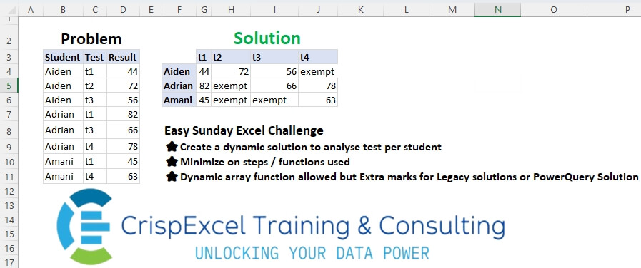
Create a dynamic solution to analyse tests per student Minimize the steps/functions used Dynamic array function allowed, but Extra marks for Legacy solutions or PowerQuery Solution
📌 Challenge Details and Links
Challenge Number: 36
Challenge Difficulty: ⭐
📥Link to the solutions on LinkedIn
Solving the challenge of Dynamic Pivot Data with Power Query
Power Query solution 1 for Dynamic Pivot Data, proposed by Zoran Milokanović:
let
  Source = Excel.CurrentWorkbook(){[Name = "Input"]}[Content],
  D = each List.Distinct(_(Source)),
  S = Table.FromRows(
    List.TransformMany(
      D(each [Student]),
      each {D(each [Test])},
      (i, _) => {i} & List.Transform(_, each Source{[Student = i, Test = _]}?[Result]? ?? "exempt")
    ),
    {" "} & D(each [Test])
  )
in
  S
Power Query solution 2 for Dynamic Pivot Data, proposed by Aditya Kumar Darak 🇮🇳:
let
  Source = Excel.CurrentWorkbook(){[Name = "data"]}[Content],
  Pivot = Table.Pivot(Source, List.Distinct(Source[Test]), "Test", "Result", each _{0}? ?? "Exempt"),
  Return = Table.Sort(Pivot, each List.PositionOf(Source[Student], [Student]))
in
  Return
Power Query solution 3 for Dynamic Pivot Data, proposed by Alejandro Simón 🇵🇦 🇪🇸:
let
  Source = Excel.CurrentWorkbook(){[Name = "Table1"]}[Content],
  Pivot = Table.Pivot(Source, List.Distinct(Source[Test]), "Test", "Result"),
  Rep = Table.ReplaceValue(Pivot, null, "exempt", Replacer.ReplaceValue, Table.ColumnNames(Pivot)),
  Sol = Table.Sort(Rep, {each List.PositionOf(List.Distinct(Source[Student]), [Student])})
in
  Sol
Power Query solution 4 for Dynamic Pivot Data, proposed by Alejandro Simón 🇵🇦 🇪🇸:
let
  Source = Excel.CurrentWorkbook(){[Name = "Table1"]}[Content],
  Test = List.Distinct(Source[Test]),
  Group = Table.Group(
    Source,
    {"Student"},
    {
      {
        "A",
        each
          let
            a = _[[Test], [Result]],
            b = Table.PromoteHeaders(Table.FromRows(Table.ToColumns(a)))
          in
            b
      }
    }
  ),
  Expand = Table.ExpandTableColumn(Group, "A", Test),
  Sol = Table.ReplaceValue(Expand, null, "exempt", Replacer.ReplaceValue, Test)
in
  Sol
Power Query solution 5 for Dynamic Pivot Data, proposed by Brian Julius:
let
  Source = Table.TransformColumnTypes(
    Excel.CurrentWorkbook(){[Name = "Table1"]}[Content],
    {"Result", Text.Type}
  ),
  Pivot = Table.Pivot(Source, List.Distinct(Source[Test]), "Test", "Result"),
  ReplNulls = Table.ReplaceValue(
    Pivot,
    null,
    "exempt",
    Replacer.ReplaceValue,
    Table.ColumnNames(Pivot)
  )
in
  ReplNulls
Power Query solution 6 for Dynamic Pivot Data, proposed by Ramiro Ayala Chávez:
let
  S = Excel.CurrentWorkbook(){[Name = "Table1"]}[Content],
  a = Table.Pivot(S, List.Distinct(S[Test]), "Test", "Result", List.Sum),
  b = Table.TransformColumnTypes(
    a,
    {{"t1", type text}, {"t2", type text}, {"t3", type text}, {"t4", type text}}
  ),
  c = Table.ReplaceValue(b, null, "exempt", Replacer.ReplaceValue, {"t1", "t2", "t3", "t4"}),
  d = Table.ToRows(c),
  e = Table.FromRows({d{1}} & {d{0}} & {d{2}}, Table.ColumnNames(c)),
  Sol = Table.RenameColumns(e, {"Student", " "})
in
  Sol
Power Query solution 7 for Dynamic Pivot Data, proposed by 🇮🇷 Navid Esmaeilzadeh اسماعیل زاده:
let
  S = Excel.CurrentWorkbook(){[Name = "Table1"]}[Content],
  A = Table.TransformColumnTypes(
    S,
    {{"Student", type text}, {"Test", type text}, {"Result", Int64.Type}}
  ),
  B = Table.Distinct(Table.SelectColumns(A, {"Student"})),
  C = Table.AddColumn(B, "Test", each List.Sort(List.Distinct(A[Test]))),
  D = Table.ExpandListColumn(C, "Test"),
  E = Table.NestedJoin(D, {"Student", "Test"}, A, {"Student", "Test"}, "C"),
  F = Table.ExpandTableColumn(E, "C", {"Result"}, {"Result"}),
  G = Table.TransformColumnTypes(F, {{"Result", type text}}),
  H = Table.ReplaceValue(G, null, "exempt", Replacer.ReplaceValue, {"Result"}),
  Sol = Table.Pivot(H, List.Distinct(H[Test]), "Test", "Result")
in
  Sol
Power Query solution 8 for Dynamic Pivot Data, proposed by Yaroslav Drohomyretskyi:
let
  Source = Excel.CurrentWorkbook(){[Name = "Table1"]}[Content],
  Result = Table.ReplaceValue(
    Table.Sort(
      Table.Pivot(Source, List.Distinct(Source[Test]), "Test", "Result", List.Sum),
      each List.PositionOf(Source[Student], [Student])
    ),
    null,
    "exempt",
    Replacer.ReplaceValue,
    List.Distinct(Source[Test])
  )
in
  Result
Power Query solution 9 for Dynamic Pivot Data, proposed by Ernesto Vega Castillo:
let
  Source = Table.TransformColumnTypes(
    Excel.CurrentWorkbook(){[Name = "Table1"]}[Content],
    {{"Test", Text.Type}, {"Result", Number.Type}}
  ),
  Sol = Table.ReplaceValue(
    Table.Pivot(Source, List.Distinct(Source[Test]), "Test", "Result"),
    null,
    "exempt",
    Replacer.ReplaceValue,
    {"t1", "t2", "t3", "t4"}
  )
in
  Sol
Power Query solution 10 for Dynamic Pivot Data, proposed by Nelson Mwangi:
let
  Source = Excel.CurrentWorkbook(){[Name = "Table1"]}[Content],
  NewTable = Table.Distinct(
    Table.SelectColumns(
      Table.AddColumn(Source, "TestList", each List.Distinct(Source[Test])),
      {"Student", "TestList"}
    ),
    "Student"
  ),
  ExpandTable = Table.ExpandListColumn(NewTable, "TestList"),
  Merge = Table.NestedJoin(
    ExpandTable,
    {"TestList", "Student"},
    Source,
    {"Test", "Student"},
    "ExpandTable",
    JoinKind.LeftOuter
  ),
  ExpandMerge = Table.ExpandTableColumn(Merge, "ExpandTable", {"Result"}, {"Result"}),
  Replacenull = Table.ReplaceValue(ExpandMerge, null, "Excempt", Replacer.ReplaceValue, {"Result"}),
  Pivot = Table.Pivot(Replacenull, List.Distinct(Replacenull[TestList]), "TestList", "Result")
in
  Pivot
Power Query solution 11 for Dynamic Pivot Data, proposed by Marc Wring:
let
  Source = Excel.CurrentWorkbook(){[Name = "tbl_data"]}[Content],
  #"Join with student_id_table" = Table.NestedJoin(
    Source,
    {"Student"},
    student_id_table,
    {"Student"},
    "student_id_table",
    JoinKind.LeftOuter
  ),
  #"Get Student ID" = Table.ExpandTableColumn(
    #"Join with student_id_table",
    "student_id_table",
    {"ID"},
    {"ID"}
  ),
  #"Pivoted Column" = Table.Pivot(
    #"Get Student ID",
    List.Distinct(#"Get Student ID"[Test]),
    "Test",
    "Result"
  ),
  #"Changed Type" = Table.TransformColumnTypes(
    #"Pivoted Column",
    {
      {"t1", type text},
      {"Student", type text},
      {"t2", type text},
      {"t3", type text},
      {"t4", type text},
      {"ID", Int64.Type}
    }
  ),
  #"Sorted ID" = Table.Sort(#"Changed Type", {{"ID", Order.Ascending}}),
  #"Remove ID column" = Table.RemoveColumns(#"Sorted ID", {"ID"}),
  #"Replaced nulls with exempt" = Table.ReplaceValue(
    #"Remove ID column",
    null,
    "exempt",
    Replacer.ReplaceValue,
    {"t1", "t2", "t3", "t4"}
  )
in
  #"Replaced nulls with exempt"
Solving the challenge of Dynamic Pivot Data with Excel
Excel solution 1 for Dynamic Pivot Data, proposed by محمد حلمي:
=LET(
   b,
   B4:B11,
   c,
   C4:C11,
   v,
   UNIQUE(
       b),

   r,
   TOROW(
       UNIQUE(
           c)),
   HSTACK(
       VSTACK(
           "",
           v),
       VSTACK(
           r,

           XLOOKUP(
               v&r,
               b&c,
               D4:D11,
               "exempt"))))
Excel solution 2 for Dynamic Pivot Data, proposed by Julian Poeltl:
=LET(
   B,
   B4:B11,
   C,
   C4:C11,
   U,
   TOROW(
       UNIQUE(
           C)),
   S,
   UNIQUE(
       B),
   VSTACK(
       HSTACK(
           "",
           U),
       HSTACK(
           S,
           XLOOKUP(
               U&S,
               C&B,
               D4:D11,
               "exempt"))))
Excel solution 3 for Dynamic Pivot Data, proposed by Oscar Mendez Roca Farell:
=LET(
   u,
    UNIQUE(
        B4:B11),
    t,
    "t"&{1,
    2 ,
    3,
    4},
    s,
    SUMIFS(
        D4:D11,
         B4:B11,
         u,
         C4:C11,
         t),
    HSTACK(
        VSTACK(
            "",
             u),
         VSTACK(
             t,
              IFERROR(
                  1/s^-1,
                   "exempt"))))
Excel solution 4 for Dynamic Pivot Data, proposed by Sunny Baggu:
=LET(

    _s,
    UNIQUE(
        B4:B11),

    _t,
    TOROW(
        UNIQUE(
            C4:C11)),

    _v,
    XLOOKUP(
        _s & _t,
         B4:B11 & C4:C11,
         D4:D11,
         "exempt"),

    VSTACK(
        HSTACK(
            "",
             _t),
         HSTACK(
             _s,
              _v))
   )
Excel solution 5 for Dynamic Pivot Data, proposed by Sunny Baggu:
=LET(

    _s,
    UNIQUE(
        B4:B11),

    _t,
    TOROW(
        UNIQUE(
            C4:C11)),

    _v,
    MAP(
        _s & _t,
         LAMBDA(
             a,
              FILTER(
                  D4:D11,
                   B4:B11 & C4:C11 = a,
                   "exempt"))),

    VSTACK(
        HSTACK(
            "",
             _t),
         HSTACK(
             _s,
              _v))
   )
Excel solution 6 for Dynamic Pivot Data, proposed by Sunny Baggu:
=LET(
_s,
    UNIQUE(
        B4:B11),

_t,
    TOROW(
        UNIQUE(
            C4:C11)),

v,
    MAKEARRAY(
ROWS(
    _s),

COLUMNS(
    _t),

LAMBDA(r,
    c,

INDEX(
BYCOL(
(B4:B11 = INDEX(
    _s,
     r,
     1)) * (C4:C11 = _t) * D4:D11,

LAMBDA(
    a,
     MAX(
         a))),

c))),

VSTACK(
    HSTACK(
        "",
         _t),
     HSTACK(
         _s,
          IF(
              v,
               v,
               "exempt"))))
Excel solution 7 for Dynamic Pivot Data, proposed by Abdallah Ally:
=IFNA(
   XLOOKUP(
       F4:F6&G3:J3,
       B4:B11&C4:C11,
       D4:D11),
   "exempt")
Excel solution 8 for Dynamic Pivot Data, proposed by Abdallah Ally:
=VSTACK(
   HSTACK(
       "",
       G3:J3),
   HSTACK(
       UNIQUE(
           B4:B11),
       IFNA(
            XLOOKUP(
                F4:F6&G3:J3,
                B4:B11&C4:C11,
                D4:D11),
           "exempt")))
Excel solution 9 for Dynamic Pivot Data, proposed by Abdallah Ally:
=LET(
   a,
   B4:B11,
   b,
   C4:C11,
   c,
   UNIQUE(
       a),
   d,
   TOROW(
       UNIQUE(
           b)),
   VSTACK(
        HSTACK(
            "",
            d),
       HSTACK(
           c,
           IFNA(
               XLOOKUP(
                   c&d,
                   a&b,
                   D4:D11),
               "exempt"))))
Excel solution 10 for Dynamic Pivot Data, proposed by Md. Zohurul Islam:
=LET(

    A,
    B4:B11,

    B,
    C4:C11,

    LokupArray,
    A & B,

    RetrnArray,
    D4:D11,

    Stdnts,
    UNIQUE(
        A),

    Tests,
    TRANSPOSE(
        UNIQUE(
            B)),

    Scores,
    XLOOKUP(

         Stdnts & Tests,

         LokupArray,

         RetrnArray,

         "exempt"
         ),

    D,
    VSTACK(
        Tests,
         Scores),

    HSTACK(
        VSTACK(
            "Students",
             Stdnts),
         D)
   )
Excel solution 11 for Dynamic Pivot Data, proposed by Asheesh Pahwa:
=DROP(
   REDUCE(
       "",
       TOROW(
           UNIQUE(
               C4:C11)),
       LAMBDA(
           x,
           y,

           HSTACK(
               x,
               LET(
                   f,
                   FILTER(
                       HSTACK(
                           B4:B11,
                           D4:D11),
                       C4:C11=y),

                   DROP(
                       REDUCE(
                           "",
                           UNIQUE(
                               B4:B11),
                           LAMBDA(
                               a,
                               v,
                               VSTACK(
                                   a,
                                   FILTER(
                                       TAKE(
                                           f,
                                           ,
                                           -1),
                                       TAKE(
                                           f,
                                           ,
                                           1)=v,
                                       "Exempt")))),
                       1))))),
   ,
   1)
Excel solution 12 for Dynamic Pivot Data, proposed by Asheesh Pahwa:
=LET(
   s,
   B4:B11,
   t,
   C4:C11,
   r,
   D4:D11,

   us,
   UNIQUE(
       s),
   ut,
   TOROW(
       UNIQUE(
           t)),

   c,
   us&ut,
   VSTACK(
       HSTACK(
           "",
           ut),
       HSTACK(
           us,
           XLOOKUP(
               c,
               s&t,
               r,
               "Exempt"))))
Excel solution 13 for Dynamic Pivot Data, proposed by Ankur Sharma:
=LET(
   a,
    B4:B11,
    b,
    UNIQUE(
        a),
    c,
    C4:C11,
    d,
    TRANSPOSE(
        UNIQUE(
            c)),
    VSTACK(
        HSTACK(
            "",
             d),
         HSTACK(
             b,
              XLOOKUP(
                  b & d,
                   a & c,
                   D4:D11,
                   "Exempt"))))
Excel solution 14 for Dynamic Pivot Data, proposed by Meganathan Elumalai:
=LET(
   s,
   B4:B11,
   t,
   C4:C11,
   r,
   UNIQUE(
       s),
   c,
   TOROW(
       UNIQUE(
           t)),
   HSTACK(

       VSTACK(
           "Name",
           r),
       VSTACK(
           c,
           XLOOKUP(
               r&"|"&c,
               s&"|"&t,
               D4:D11,

               "Exempt"))))
Excel solution 15 for Dynamic Pivot Data, proposed by Meganathan Elumalai:
=INDEX(
   $B$4:$B$11,
   MODE.MULT(
       IFERROR(
           MATCH(
               ROW(
                   $B$4:$B$11)-ROW(
                   $B$4)+1,
               MATCH(
                   $B$4:$B$11,
                   $B$4:$B$11,
                   0),
               {0,
               0}),
           "")))
For Column Headers,

=TRANSPOSE(
   INDEX(
       $C$4:$C$11,
       MODE.MULT(
           IFERROR(
               MATCH(
                   ROW(
                       $C$4:$C$11)-ROW(
                       $C$4)+1,
                   MATCH(
                       $C$4:$C$11,
                       $C$4:$C$11,
                       0),
                   {0,
                   0}),
               "")))),

for Results,

=IFERROR(
   VLOOKUP(
       $F4&"|"&G$3,
       CHOOSE(
           {1,
           2},
           $B$4:$B$11&"|"&$C$4:$C$11,
           $D$4:$D$11),
       2,
       0),
   "exempt")
Excel solution 16 for Dynamic Pivot Data, proposed by Mey Tithveasna:
=LET(
   b,
   B4:B11,
   c,
   C4:C11,
   u,
   UNIQUE(
       b),
   r,
   TOROW(
       UNIQUE(
           c)),
   VSTACK(
       HSTACK(
           "",
           r),
       HSTACK(
           u,
           XLOOKUP(
               F4:F6&r,
               b&c,
               D4:D11,
               "exempt"))))
Excel solution 17 for Dynamic Pivot Data, proposed by Mey Tithveasna:
=IFNA(
   INDEX(
       $D$4:$D$11,

       XMATCH(
           $F4&G$3,

           $B$4:$B$11&$C$4:$C$11,
           )),
   "exempt")
Excel solution 18 for Dynamic Pivot Data, proposed by Milan Shrimali:
GOOGLESHEETS SOLUTIONS :
LET(
   STD,
   UNIQUE(
       B4:B11),
   TST,
   TRANSPOSE(
       UNIQUE(
           C4:C11)),
   IFERROR(
       HSTACK(
           VSTACK(
               " ",
               STD),
           VSTACK(
               TST,

               BYROW(
                   STD,
                   LAMBDA(
                       X,
                       ARRAYFORMULA(
                           XLOOKUP(
                               X&BYCOL(
                                   TST,
                                   LAMBDA(
                                       X,
                                       X)),
                               B4:B11&C4:C11,
                               D4:D11)))))),
       "EXEMPT"))
Excel solution 19 for Dynamic Pivot Data, proposed by Tomasz Jakóbczyk:
=LET(
   x,
   UNIQUE(
       $B$4:$B$11),
   y,
   TRANSPOSE(
       SORT(
           UNIQUE(
               $C$4:$C$11))),
   HSTACK(
       VSTACK(
           "",
           x),
       VSTACK(
           y,
           XLOOKUP(
               x&"|"&y,
               $B$4:$B$11&"|"&$C$4:$C$11,
               $D$4:$D$11,
               "exempt"))))

Second way:
For row headers: =UNIQUE(
   B4:B11)
For column headers: =TRANSPOSE(
   UNIQUE(
       SORT(
           C4:C11)))
For results: =FILTER($D$4:$D$11,
   ($C$4:$C$11=G$3)*($B$4:$B$11=$F4),
   "exempt")
Solving the challenge of Dynamic Pivot Data with Python
Python solution 1 for Dynamic Pivot Data, proposed by Konrad Gryczan, PhD:
import pandas as pd
path = "files/Excel Challange 28th July.xlsx"
input = pd.read_excel(path, usecols="B:D", skiprows=2, dtype=str)
test = pd.read_excel(path, usecols="F:J", skiprows=2, nrows=3, dtype=str)
test.columns = ["Student", "t1", "t2", "t3", "t4"]
test = test.sort_values(by="Student").reset_index(drop=True)
result = input.pivot(index="Student", columns="Test", values="Result").fillna("exempt").reset_index()
result.columns.name = None
print(result.equals(test)) # True
Solving the challenge of Dynamic Pivot Data with Python in Excel
Python in Excel solution 1 for Dynamic Pivot Data, proposed by Abdallah Ally:
df = xl("B3:D11", headers=True)
# Perform data munging
df['ind'] = (df['Student'] != df['Student'].shift(1)).cumsum()
df = df.pivot(
 index=['ind', 'Student'], columns='Test', values='Result'
).reset_index().fillna('exempt')
df = df.iloc[:, 1:]
df.columns = [''] + df.columns[1:].tolist()
df
Python in Excel solution 2 for Dynamic Pivot Data, proposed by Owen Price:
pandas pivot table with
#pythoninexcel
Solving the challenge of Dynamic Pivot Data with R
R solution 1 for Dynamic Pivot Data, proposed by Konrad Gryczan, PhD:
library(tidyverse)
library(readxl)
path = "files/Excel Challange 28th July.xlsx"
input = read_excel(path, range = "B3:D11", col_types = "text")
test = read_excel(path, range = "F3:J6", col_types = "text")
colnames(test) = c("Student", "t1", "t2", "t3", "t4")
result = input %>%
 pivot_wider(names_from = "Test", values_from = "Result", values_fill = "exempt")
identical(result, test)
# [1] TRUE